Practice of Large Model Training Process

6.1 Model Pretraining

In the previous chapter, we gradually decomposed the model structure and training process of LLM, implemented the LLaMA model structure and the entire Pretrain and SFT process from scratch, and gained a deeper understanding of the principles and training details of LLM. However, in practical applications, implementing LLM training manually has the following problems:

• Manually implementing LLM structures is labor-intensive and difficult to keep up with the latest structural innovations;
• Implementing LLM training from scratch cannot effectively achieve multi-card distributed training, resulting in low training efficiency;
• Incompatible with existing pre-trained LLMs, unable to use pre-trained model parameters

Therefore, in this chapter, we will introduce the mainstream training framework Transformers in the LLM field, and combine it with mainstream frameworks such as distributed framework deepspeed and efficient fine-tuning framework peft, to practice using transformers for the entire Pretrain and SFT process, thereby better connecting to industry's mainstream LLM technical solutions.

6.1.1 Framework Introduction

Transformers is an NLP framework developed by Hugging Face, which provides unified support for over a hundred mainstream model architectures such as BERT, GPT, LLaMA, T5, and ViT through a modular design. By using Transformers, developers do not need to repeatedly implement basic network structures, and can load any pre-trained model with one click via the AutoModel class.

At the same time, the built-in Trainer class encapsulates the core logic of distributed training, supporting multiple distributed training strategies such as PyTorch native DDP, DeepSpeed, and Megatron-LM. By simply configuring training parameters, data parallelism, model parallelism, and pipeline parallelism can be achieved, and efficient training of billion-parameter models can be easily supported on an 8-card A100 cluster. Combined with components such as SavingPolicy and LoggingCallback, the training process is automated. It also supports integration with frameworks such as Deepspeed, peft, wandb, and Swanlab, and can seamlessly connect directly through parameter settings, thus quickly and efficiently achieving LLM training.

More importantly for NLP researchers in the LLM era, HuggingFace has built its vast AI community based on the Transformers framework, opening up hundreds of millions of pre-trained model parameters and 250,000+ different types of datasets. Through the integration of multiple frameworks such as Transformers, Dataset, and Evaluate, it helps developers conveniently use any pre-trained model, and conveniently develop and apply their own models on the basis of open-source models and datasets.

In the LLM era, adjusting model structures and re-pretraining are becoming less frequent, and more business applications focus on using pre-trained LLMs for Post Train and SFT to support their downstream business applications. Moreover, due to the large size of pre-trained models, it has gradually become an essential skill to conveniently integrate distributed training frameworks like deepspeed in the LLM era. Therefore, Transformers have gradually become the mainstream framework for NLP technology in both academia and industry. Whether it is enterprise business development or scientific research, Transformers are increasingly the preferred choice for model implementation. At the same time, newly released open-source LLMs such as DeepSeek and Qwen also open up their pre-trained weights and model calling demos in the Transformers community immediately. By using the Transformers framework, LLM training and development can be efficiently and conveniently completed, achieving industrial-level output delivery. Next, we will introduce how to implement LLM Pretrain and SFT based on the Transformers framework.

6.1.2 Initialize LLM

We can directly initialize an already implemented model using the AutoModel class of Transformers. Any pre-trained model contains configuration information about the model in its parameters. If you want to train an LLM from scratch, you can directly initialize it using an existing model architecture.

We can use the configuration information of this model to initialize a Qwen-2.5-1.5B model for training, or make changes to the configuration information, such as modifying the hidden layer size, the number of attention heads, etc., to customize a model structure. HuggingFace provides a Python tool to conveniently download the model parameters you want to use:

import os
# Set environment variables, here using HuggingFace mirror website
os.environ['HF_ENDPOINT'] = 'https://hf-mirror.com'
# Download model
os.system('huggingface-cli download --resume-download Qwen/Qwen2.5-1.5B --local-dir your_local_dir')

After downloading, you can directly load the downloaded configuration file using the AutoConfig class:

# Load the defined model parameters - taking Qwen-2.5-1.5B as an example
# Use the Config class of transforemrs to load
from transformers import AutoConfig

# Local path of the downloaded parameters
model_path = "qwen-1.5b"
config = AutoConfig.from_pretrained(model_name_or_path)

You can also customize the configuration file and load it in the same way. You can use the AutoModel class to generate the corresponding model based on the loaded configuration object:

# Generate a defined model using this configuration
from transformers import AutoModelForCausalLM

model = AutoModelForCausalLM.from_config(config, trust_remote_code=True)

Since LLMs are generally CausalLM architectures, the AutoModelForCausalLM class is used for loading. If it is used for classification task training, the AutoModelForSequenceClassification class can be used for loading. Viewing this model, as shown in Figure 6.6, its architecture is the same as the defined configuration file:

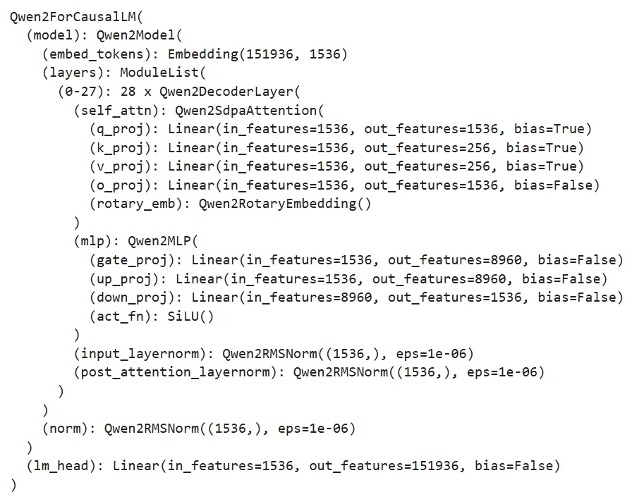
Figure 6.6 Model Structure Output Result

This model is a Qwen-2.5-1.5B model initialized from scratch. Usually, we rarely pretrain LLMs from scratch, and most practices involve loading a pre-trained LLM weight and then post-training on our corpus. Here, we also introduce how to initialize a pre-trained model from the downloaded model parameters.

from transformers import AutoModelForCausalLM

model = AutoModelForCausalLM.from_pretrained(model_name_or_path, trust_remote_code=True)

Similarly, directly use the from_pretrained method to load. Here, the model_name_or_path is the local path of the downloaded parameters.

We also need to initialize a tokenizer. Here, we directly use the tokenizer parameters corresponding to Qwen-2.5-1.5B:

# Load a pre-trained tokenizer
from transformers import AutoTokenizer

tokenizer = AutoTokenizer.from_pretrained(model_name_or_path)

The loaded tokenizer can be used directly, and can perform tokenization on any text.

6.1.3 Pretraining Data Processing

Similar to Chapter 5, we use the Mobvoi sequence monkey open dataset as the pretraining dataset, and can download and extract the dataset in the same way as in Chapter 5. The datasets library of HuggingFace is a third-party library that comes with the Transformers framework for data download and processing. We can directly use the load_dataset function of datasets to load the pretraining data:

# Load pretraining data
from datasets import load_dataset

ds = load_dataset('json', data_files='/mobvoi_seq_monkey_general_open_corpus.jsonl')

Note that due to the large size of the dataset, loading may take a long time or cause memory issues. It is recommended to split part of the pretraining dataset for testing during the initial phase. The loaded ds is a DatasetDict object, and the data is saved by default in the value corresponding to the 'train' key. You can view it with the following code:

ds["train"][0]

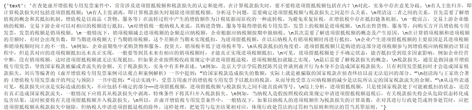
Figure 6.7 Dataset Display

You can view the features (i.e., columns) of the dataset using the feature attribute. Here, we need to save the column names of the dataset because after tokenizing the text, we need to remove the original text:

# View features
column_names = list(ds["train"].features)
# columnes_name: ["text"]

Next, process the dataset using the loaded tokenizer. Here, we use the map function for batch processing:

# Tokenize the dataset
def tokenize_function(examples):
    # Use the preloaded tokenizer for tokenization
    output = tokenizer([item for item in examples["text"]])
    return output

# Batch processing
tokenized_datasets = ds.map(
    tokenize_function,
    batched=True,
    num_proc=10,
    remove_columns=column_names,
    load_from_cache_file=True,
    desc="Running tokenizer on dataset",
)

The processed dataset will include 'input_ids' and 'attention_mask' columns, which are the numerical sequences and attention masks (indicating whether padding is present) after tokenizing the text. The map method will remove the original 'text' via the remove_columns parameter, and it will not be used during training.

Since pretraining is generally a CLM task, learning the sequential semantics of multiple samples at once does not affect model performance, and the training data is large and training time is long, requiring high training efficiency. During the pretraining process, multiple text segments are usually concatenated together, processed into a uniform length text block, and then each text block is trained. Here, we implement a concatenation function to concatenate the text blocks to a length of 2048 tokens, and then perform batch processing via the map method:

# Pretraining generally concatenates text into fixed-length text segments
from itertools import chain

# Here we take the block length as 2048
block_size = 2048

def group_texts(examples):
    # Concatenate the text segments
    concatenated_examples = {k: list(chain(*examples[k])) for k in examples.keys()}
    # Calculate the total length of the concatenated result
    total_length = len(concatenated_examples[list(examples.keys())[0]])
    # If the length is too long, split it
    if total_length >= block_size:
        total_length = (total_length // block_size) * block_size
    # Split by block_size
    result = {
        k: [t[i : i + block_size] for i in range(0, total_length, block_size)]
        for k, t in concatenated_examples.items()
    }
    # For CLM tasks, labels and input are the same
    result["labels"] = result["input_ids"].copy()
    return result

# Batch processing
lm_datasets = tokenized_datasets.map(
    group_texts,
    batched=True,
    num_proc=10,
    load_from_cache_file=True,
    desc=f"Grouping texts in chunks of {block_size}",
    batch_size = 40000,
)
train_dataset = lm_datasets["train"]

The processed train_dataset is a pretraining dataset directly usable for CLM Pretrain, with each sample length of 2048 tokens.

6.1.4 Training Using Trainer

Next, we use the Trainer class provided by Transformers for training. The Trainer encapsulates the model training logic and has done good efficiency optimization and visualization work, which can efficiently and conveniently complete the training of LLM.

First, we need to configure the training hyperparameters, using the TrainingArguments class to instantiate a parameter object:

from transformers import TrainingArguments
# Configure training parameters

training_args = TrainingArguments(
    output_dir="output",  # Path for outputting training parameters
    per_device_train_batch_size=4,  # Batch size for training
    gradient_accumulation_steps=4,  # Number of gradient accumulation steps, actual bs = set bs * accumulation steps
    logging_steps=10,  # Step interval for printing loss
    num_train_epochs=1,  # Number of training epochs
    save_steps=100,  # Step interval for saving model parameters
    learning_rate=1e-4,  # Learning rate
    gradient_checkpointing=True  # Enable gradient checkpointing
)

Then, based on the initialized model, tokenizer, and training_args, and passing the processed training dataset, we instantiate a trainer object:

from transformers import Trainer, default_data_collator
from torchdata.datapipes.iter import IterableWrapper

# Trainer
trainer = Trainer(
    model=model,
    args=training_args,
    train_dataset=IterableWrapper(train_dataset),
    eval_dataset=None,
    tokenizer=tokenizer,
    # Default is MLM collator, use CLM collater
    data_collator=default_data_collator
)

Then, using the train method will start training and saving according to the configured training hyperparameters:

trainer.train()

Note: The above code is stored in the ./code/pretrain.ipynb file.

6.1.5 Implementing Distributed Training with DeepSpeed

Due to the large scale and long duration of pretraining, it is generally not recommended to run it in Jupyter Notebook, as it is prone to interruption. Also, due to the large scale of pretraining, it usually requires distributed training across multiple cards, otherwise the training time would be too long. Here, we introduce how to implement distributed training using the DeepSpeed framework based on the above code, thus completing industry-ready LLM Pretrain.

Long-term training usually uses bash scripts to set hyperparameters and then start the written python script for training. We use a Python script (./code/pretrain.py) to implement the entire training process.

First, import the required third-party libraries:

import logging
import math
import os
import sys
from dataclasses import dataclass, field
from torchdata.datapipes.iter import IterableWrapper
from itertools import chain
import deepspeed
from typing import Optional, List

import datasets
import pandas as pd
import torch
from datasets import load_dataset
import transformers
from transformers import (
    AutoConfig,
    AutoModelForCausalLM,
    AutoTokenizer,
    HfArgumentParser,
    Trainer,
    TrainingArguments,
    default_data_collator,
    set_seed,
)
import datetime
from transformers.testing_utils import CaptureLogger
from transformers.trainer_utils import get_last_checkpoint
import swanlab

First, define several types of hyperparameters for processing the values set in the sh script. Since Transformers itself has the TraingingArguments class, which includes some essential hyperparameters for training. We only need to define the hyperparameters not included in TrainingArguments, mainly including model-related hyperparameters (defined in ModelArguments) and data-related hyperparameters (defined in DataTrainingArguments):

# Hyperparameter class
@dataclass
class ModelArguments:
    """
    Parameters related to the model
    """

    model_name_or_path: Optional[str] = field(
        default=None,
        metadata={
            "help": (
                "Post-training usage, address of pre-trained model parameters"
            )
        },
    )
    config_name: Optional[str] = field(
        default=None, metadata={"help": "Pre-training usage, Config file address"}
    )
    tokenizer_name: Optional[str] = field(
        default=None, metadata={"help": "Pre-training Tokenizer address"}
    )
    torch_dtype: Optional[str] = field(
        default=None,
        metadata={
            "help": (
                "Data type used for model training, recommend bfloat16"
            ),
            "choices": ["auto", "bfloat16", "float16", "float32"],
        },
    )


@dataclass
class DataTrainingArguments:
    """
    Parameters related to training
    """

    train_files: Optional[List[str]]  = field(default=None, metadata={"help": "Training data path"})
    block_size: Optional[int] = field(
        default=None,
        metadata={
            "help": (
                "Set text block length"
            )
        },
    )
    preprocessing_num_workers: Optional[int] = field(
        default=None,
        metadata={"help": "Number of threads used for preprocessing."},
    )

Then, we can define a main function to encapsulate the above training process. First, we load the hyperparameters set in the sh script using the HfArgumentParser tool provided by Transformers:

# Load script parameters
parser = HfArgumentParser((ModelArguments, DataTrainingArguments, TrainingArguments))
model_args, data_args, training_args = parser.parse_args_into_dataclasses()

In large-scale training, it is generally recommended to use log to save the information of the training process, and it is not recommended to use print directly, which can lead to the loss of key training information. Here, we directly use the logging library of Python to implement log recording. First, we need to set up the log:

# Set log
logging.basicConfig(
    format="%(asctime)s - %(levelname)s - %(name)s - %(message)s",
    datefmt="%m/%d/%Y %H:%M:%S",
    handlers=[logging.StreamHandler(sys.stdout)],
)

# Set log level to INFO
transformers.utils.logging.set_verbosity_info()
log_level = training_args.get_process_log_level()
logger.setLevel(log_level)
datasets.utils.logging.set_verbosity(log_level)
transformers.utils.logging.set_verbosity(log_level)
transformers.utils.logging.enable_default_handler()
transformers.utils.logging.enable_explicit_format()

Here, the log level is set to INFO. Logging has five levels: DEBUG, INFO, WARNING, ERROR, and CRITICAL. Setting the log level to a certain level will only output information at that level and above. After setting, wherever you need to record logs, you can directly use logger, and when recording, specify the log level, for example:

# Record overall training situation
logger.warning(
    f"Process rank: {training_args.local_rank}, device: {training_args.device}, n_gpu: {training_args.n_gpu}"
    + f"distributed training: {bool(training_args.local_rank != -1)}, 16-bits training: {training_args.fp16}"
)
logger.info(f"Training/evaluation parameters {training_args}")

Subsequent logs in the script will not be detailed.

In large-scale training, it is often difficult to avoid interruptions. Training is usually set to save checkpoints at fixed intervals, and resume training from the last checkpoint after an interruption. Therefore, we need to first check whether there is an old checkpoint and resume training from the checkpoint:

# Check for checkpoints
last_checkpoint = None
if os.path.isdir(training_args.output_dir):
    # Use the get_last_checkpoint provided by transformers to automatically detect
    last_checkpoint = get_last_checkpoint(training_args.output_dir)
    if last_checkpoint is None and len(os.listdir(training_args.output_dir)) > 0:
        raise ValueError(
            f"Output path ({training_args.output_dir}) is not empty "
        )
    elif last_checkpoint is not None and training_args.resume_from_checkpoint is None:
        logger.info(
            f"Resuming training from {last_checkpoint}"
        )

Next, initialize the model as introduced earlier. Here, we wrap initializing from scratch and initializing based on an existing pre-trained model together:

# Initialize model
if model_args.config_name is not None:
    # from scratch
    config = AutoConfig.from_pretrained(model_args.config_name)
    logger.warning("You are initializing a model from scratch")
    logger.info(f"Model parameter configuration address: {model_args.config_name}")
    logger.info(f"Model parameters: {config}")
    model = AutoModelForCausalLM.from_config(config, trust_remote_code=True)
    n_params = sum({p.data_ptr(): p.numel() for p in model.parameters()}.values())
    logger.info(f"Pretraining a new model - Total size={n_params/2**20:.2f}M params")
elif model_args.model_name_or_path is not None:
    logger.warning("You are initializing a pre-trained model")
    logger.info(f"Model parameter address: {model_args.model_name_or_path}")
    model = AutoModelForCausalLM.from_pretrained(model_args.model_name_or_path, trust_remote_code=True)
    n_params = sum({p.data_ptr(): p.numel() for p in model.parameters()}.values())
    logger.info(f"Inheriting a pre-trained model - Total size={n_params/2**20:.2f}M params")
else:
    logger.error("config_name and model_name_or_path cannot both be empty")
    raise ValueError("config_name and model_name_or_path cannot both be empty")

Then, similarly load the tokenizer and preprocess the pretraining data. This part is exactly the same as above, and will not be repeated here. Readers can check the details in the code. Similarly, use the Trainer for training:

logger.info("Initializing Trainer")
trainer = Trainer(
    model=model,
    args=training_args,
    train_dataset=IterableWrapper(train_dataset),
    tokenizer=tokenizer,
    data_collator=default_data_collator
)

# Load from checkpoint
checkpoint = None
if training_args.resume_from_checkpoint is not None:
    checkpoint = training_args.resume_from_checkpoint
elif last_checkpoint is not None:
        checkpoint = last_checkpoint

logger.info("Starting training")
train_result = trainer.train(resume_from_checkpoint=checkpoint)
trainer.save_model() 

Note that since the existence of checkpoints was checked earlier, here we use resume_from_checkpoint to realize resuming training from the checkpoint.

Since monitoring the training progress and the trend of loss descent is particularly important in large-scale training, in the script, we used swanlab as the training monitoring tool. At the beginning of the script, we initialized swanlab:

# Initialize SwanLab
swanlab.init(project="pretrain", experiment_name="from_scrach")

After starting the training, the terminal will output the url monitored by swanlab, and clicking it allows you to observe the training progress. Here, we will not elaborate on the details of swanlab's usage, and readers are welcome to refer to relevant documentation.

After completing the above code, we use a sh script (./code/pretrain.sh) to define the values of various hyperparameters and start the training using Deepspeed to achieve efficient multi-card distributed training:

# Set visible GPUs
CUDA_VISIBLE_DEVICES=0,1

deepspeed pretrain.py \
    --config_name autodl-tmp/qwen-1.5b \
    --tokenizer_name autodl-tmp/qwen-1.5b \
    --train_files autodl-tmp/dataset/pretrain_data/mobvoi_seq_monkey_general_open_corpus_small.jsonl \
    --per_device_train_batch_size 16 \
    --gradient_accumulation_steps 4 \
    --do_train \
    --output_dir autodl-tmp/output/pretrain \
    --evaluation_strategy no \
    --learning_rate 1e-4 \
    --num_train_epochs 1 \
    --warmup_steps 200 \
    --logging_dir autodl-tmp/output/pretrain/logs \
    --logging_strategy steps \
    --logging_steps 5 \
    --save_strategy steps \
    --save_steps 100 \
    --preprocessing_num_workers 10 \
    --save_total_limit 1 \
    --seed 12 \
    --block_size 2048 \
    --bf16 \
    --gradient_checkpointing \
    --deepspeed ./ds_config_zero2.json \
    --report_to swanlab
    # --resume_from_checkpoint ${output_model}/checkpoint-20400 \

After installing the DeepSpeed third-party library, you can directly start multi-card training using the DeepSpeed command. The above script command mainly defines various hyperparameter values and can be referenced for use. In Chapter 4, we introduced the principle of DeepSpeed distributed training and the ZeRO stage settings. Here, we use ZeRO-2 for training. Here, we load ds_config_zero.json as the DeepSpeed configuration parameters:

{
    "fp16": {
        "enabled": "auto",
        "loss_scale": 0,
        "loss_scale_window": 1000,
        "initial_scale_power": 16,
        "hysteresis": 2,
        "min_loss_scale": 1
    },
    "bf16": {
        "enabled": "auto"
    },
    "optimizer": {
        "type": "AdamW",
        "params": {
            "lr": "auto",
            "betas": "auto",
            "eps": "auto",
            "weight_decay": "auto"
        }
    },

    "scheduler": {
        "type": "WarmupLR",
        "params": {
            "warmup_min_lr": "auto",
            "warmup_max_lr": "auto",
            "warmup_num_steps": "auto"
        }
    },

    "zero_optimization": {
        "stage": 2,
        "offload_optimizer": {
            "device": "none",
            "pin_memory": true
        },
        "allgather_partitions": true,
        "allgather_bucket_size": 2e8,
        "overlap_comm": true,
        "reduce_scatter": true,
        "reduce_bucket_size": 2e8,
        "contiguous_gradients": true
    },

    "gradient_accumulation_steps": "auto",
    "gradient_clipping": "auto",
    "steps_per_print": 100,
    "train_batch_size": "auto",
    "train_micro_batch_size_per_gpu": "auto",
    "wall_clock_breakdown": false
}

Finally, run the pretrain.sh script in the terminal to start the training.

6.2 Supervised Fine-tuning

In the previous section, we introduced how to quickly and efficiently perform model pretraining using the Transformers framework. In this section, we will build on the above content to introduce how to perform supervised fine-tuning on a pre-trained model using the Transformers framework.

6.2.1 Pretrain vs SFT

First, we need to recall what the core differences between pretraining and supervised fine-tuning of LLMs are. In Chapter 4, it was mentioned that currently formed LLMs are generally trained through three stages: Pretrain-SFT-RLHF. In the Pretrain stage, massive unsupervised texts are used for self-supervised modeling to learn the semantic rules of the text and the world knowledge in the text; in the SFT stage, the pre-trained model is usually fine-tuned with instructions, that is, the model is trained to complete corresponding tasks based on user instructions, so that the model can follow user instructions, plan, act, and output according to user instructions. Therefore, both Pretrain and SFT use CLM modeling, and their core difference lies in that Pretrain uses massive unsupervised texts for training, and the model directly performs the "predict next token" task on the entire text; while SFT uses paired instruction data, and the model models the subsequent output based on the input instruction. Reflected in specific training implementation, Pretrain calculates loss for the entire text, requiring the model to model and predict the entire text; while SFT only calculates loss for the output, without calculating loss for the instruction part.

Therefore, compared to the Pretrain code in the previous section, the SFT part only needs to modify the data processing part, building training samples from instruction pairs, and the rest is completely consistent with the implementation logic of Pretrain. The code script for this section is ./code/finetune.py.

6.2.2 Fine-tuning Data Processing

Similarly to Chapter 5, we use the BelleGroup open dataset from贝壳 for SFT.

During the SFT process, we will define a Chat Template, which represents how to convert conversation data into a text sequence that the model can fit. When using a model that has been SFT to perform downstream task fine-tuning, it is generally necessary to check the Chat Template of the model and adapt it, which is to prevent damage to the instruction-following ability learned in SFT. Since we are using a Pretrain model for SFT, we can define a custom Chat Template. Since we are using the Qwen-2.5-1.5B model structure for Pretrain, we will continue to use the Qwen-2.5 Chat Template. If readers do not have sufficient resources to perform the Pretrain of the previous part, they can also use the official Qwen-2.5-1.5B model as the base model for SFT.

We first define some special tokens. Special tokens have special roles in the model fitting process, including the beginning of the text sequence (BOS), the end of the text sequence (EOS), newline characters, etc. Defining special tokens helps avoid semantic confusion during the model fitting process:

# Different tokenizers require special definitions
# BOS
im_start = tokenizer("<|im_start|>").input_ids
# EOS
im_end = tokenizer("<|im_end|>").input_ids
# PAD
IGNORE_TOKEN_ID = tokenizer.pad_token_id
# Newline character
nl_tokens = tokenizer('\n').input_ids
# Role identifiers
_system = tokenizer('system').input_ids + nl_tokens
_user = tokenizer('human').input_ids + nl_tokens
_assistant = tokenizer('assistant').input_ids + nl_tokens

The Chat Template of the Qwen series generally has three dialogue roles: System, User, and Assistant. The System is the system prompt, responsible for activating the model's capabilities, with the default being "You are a helpful assistant." It is generally not changed during the SFT process. The User is the user's prompt, and here since the dialogue role in the dataset is "human," we have modified "user" to "human." The Assistant is the response given by the LLM, which is the text that the model needs to fit during the SFT process.

Next, since this dataset is a multi-turn dialogue dataset, we need to process the multi-turn dialogues and concatenate them into a single text sequence:

# Concatenate multi-turn dialogues
input_ids, targets = [], []
# Multiple samples
for i in tqdm(range(len(sources))):
    # source is a multi-turn dialogue sample
    source = sources[i]
    # Start from user
    if source[0]["from"] != "human":
        source = source[1:]
    # Input and output respectively
    input_id, target = [], []
    # system: 【BOS】system\nYou are a helpful assistant.【EOS】\n
    system = im_start + _system + tokenizer(system_message).input_ids + im_end + nl_tokens
    input_id += system
    # system does not need to be fitted
    target += im_start + [IGNORE_TOKEN_ID] * (len(system)-3) + im_end + nl_tokens
    assert len(input_id) == len(target)
    # Concatenate sequentially
    for j, sentence in enumerate(source):
        # Sentence is a round of dialogue
        role = roles[sentence["from"]]
        # user：<|im_start|>human\ninstruction【EOS】\n
        # assistant：<|im_start|>assistant\nresponse【EOS】\n
        _input_id = tokenizer(role).input_ids + nl_tokens + \
            tokenizer(sentence["value"]).input_ids + im_end + nl_tokens
        input_id += _input_id
        if role == '<|im_start|>human':
            # user does not need to be fitted
            _target = im_start + [IGNORE_TOKEN_ID] * (len(_input_id)-3) + im_end + nl_tokens
        elif role == '<|im_start|>assistant':
            # assistant needs to be fitted
            _target = im_start + [IGNORE_TOKEN_ID] * len(tokenizer(role).input_ids) + \
                _input_id[len(tokenizer(role).input_ids)+1:-2] + im_end + nl_tokens
        else:
            print(role)
            raise NotImplementedError
        target += _target
    assert len(input_id) == len(target)
    # Finally, perform PAD
    input_id += [tokenizer.pad_token_id] * (max_len - len(input_id))
    target += [IGNORE_TOKEN_ID] * (max_len - len(target))
    input_ids.append(input_id[:max_len])
    targets.append(target[:max_len])

The above code follows the Qwen Chat Template logic, and readers can also modify it according to their preferences. The core point is that the user's text does not need to be fitted, so the corresponding text content in targets is masked with IGNORE_TOKEN_ID, while the assistant's text content is the original text, which needs to calculate the loss. Currently, the majority of LLMs set IGNORE_TOKEN_ID to -100.

After concatenation, convert the tokenized numerical sequence into Torch.tensor, and then concatenate it into a dictionary required by Dataset:

input_ids = torch.tensor(input_ids)
targets = torch.tensor(targets)

return dict(
    input_ids=input_ids,
    labels=targets,
    attention_mask=input_ids.ne(tokenizer.pad_token_id),
)

After completing the above processing logic, we need to define a Dataset class, which calls this logic for data processing in the class:

class SupervisedDataset(Dataset):

    def __init__(self, raw_data, tokenizer, max_len: int):
        super(SupervisedDataset, self).__init__()
        # Load and preprocess data
        sources = [example["conversations"] for example in raw_data]
        # preprocess is the data preprocessing logic defined above
        data_dict = preprocess(sources, tokenizer, max_len)

        self.input_ids = data_dict["input_ids"]
        self.labels = data_dict["labels"]
        self.attention_mask = data_dict["attention_mask"]

    def __len__(self):
        return len(self.input_ids)

    def __getitem__(self, i) -> Dict[str, torch.Tensor]:
        return dict(
            input_ids=self.input_ids[i],
            labels=self.labels[i],
            attention_mask=self.attention_mask[i],
        )

This class inherits from the Dataset class of Torch and can be directly used in the Trainer. After data processing, modify the data processing logic based on the previous script, and the subsequent model training is almost completely consistent. Here is the main function logic:

# Load script parameters
parser = HfArgumentParser((ModelArguments, DataTrainingArguments, TrainingArguments))
model_args, data_args, training_args = parser.parse_args_into_dataclasses()

# Initialize SwanLab
swanlab.init(project="sft", experiment_name="qwen-1.5b")

# Set log
logging.basicConfig(
    format="%(asctime)s - %(levelname)s - %(name)s - %(message)s",
    datefmt="%m/%d/%Y %H:%M:%S",
    handlers=[logging.StreamHandler(sys.stdout)],
)

# Set log level to INFO
transformers.utils.logging.set_verbosity_info()
log_level = training_args.get_process_log_level()
logger.setLevel(log_level)
datasets.utils.logging.set_verbosity(log_level)
transformers.utils.logging.set_verbosity(log_level)
transformers.utils.logging.enable_default_handler()
transformers.utils.logging.enable_explicit_format()

# Record overall training situation
logger.warning(
    f"Process rank: {training_args.local_rank}, device: {training_args.device}, n_gpu: {training_args.n_gpu}"
    + f"distributed training: {bool(training_args.local_rank != -1)}, 16-bits training: {training_args.fp16}"
)
logger.info(f"Training/evaluation parameters {training_args}")

# Check checkpoint
last_checkpoint = None
if os.path.isdir(training_args.output_dir):
    last_checkpoint = get_last_checkpoint(training_args.output_dir)
    if last_checkpoint is None and len(os.listdir(training_args.output_dir)) > 0:
        raise ValueError(
            f"Output path ({training_args.output_dir}) is not empty "
        )
    elif last_checkpoint is not None and training_args.resume_from_checkpoint is None:
        logger.info(
            f"Resuming training from {last_checkpoint}"
        )

# Set random seed.
set_seed(training_args.seed)

# Initialize model
logger.warning("Loading pre-trained model")
logger.info(f"Model parameter address: {model_args.model_name_or_path}")
model = AutoModelForCausalLM.from_pretrained(model_args.model_name_or_path, trust_remote_code=True)
n_params = sum({p.data_ptr(): p.numel() for p in model.parameters()}.values())
logger.info(f"Inheriting a pre-trained model - Total size={n_params/2**20:.2f}M params")

# Initialize Tokenizer
tokenizer = AutoTokenizer.from_pretrained(model_args.model_name_or_path)
logger.info("Completed tokenizer loading")

# Load fine-tuning data
with open(data_args.train_files) as f:
    lst = [json.loads(line) for line in f.readlines()[:10000]]
logger.info("Completed training set loading")
logger.info(f"Training set address: {data_args.train_files}")
logger.info(f'Number of training samples: {len(lst)}')
# logger.info(f"Training set sample: {ds["train"][0]}")

train_dataset = SupervisedDataset(lst, tokenizer=tokenizer, max_len=2048)

logger.info("Initializing Trainer")
trainer = Trainer(
    model=model,
    args=training_args,
    train_dataset= IterableWrapper(train_dataset),
    tokenizer=tokenizer
)

# Load from checkpoint
checkpoint = None
if training_args.resume_from_checkpoint is not None:
    checkpoint = training_args.resume_from_checkpoint
elif last_checkpoint is not None:
        checkpoint = last_checkpoint

logger.info("Starting training")
train_result = trainer.train(resume_from_checkpoint=checkpoint)
trainer.save_model() 

The startup method is also started using deepspeed in the sh script, and will not be detailed here. The source code can be found in ./code/finetune.sh.

6.3 Efficient Fine-tuning

In the previous sections, we have detailed the principles and practical details of performing Pretrain, SFT, and RLHF on models based on the Transformers framework. However, due to the large number of parameters in LLMs and the large amount of training data, training the model using the above methods (mainly SFT and RLHF) requires adjusting all model parameters, which puts a huge resource pressure on enterprises or research groups with limited resources. How to efficiently and quickly fine-tune the model for domain or task-specific purposes, and use LLM to accomplish target tasks at a low cost, is very important.

6.3.1 Efficient Fine-tuning Solutions

To address the high cost of full fine-tuning, there are currently two main solutions:

Adapt Tuning. That is, adding an Adapter layer to the model, freezing the original parameters during fine-tuning, and only updating the Adapter layer.

Specifically, it inserts a parameter for the downstream task into each layer of the pre-trained model, i.e., the Adapter module, and freezes the model body during fine-tuning, only training the parameters specific to the task, as shown in Figure 6.8.

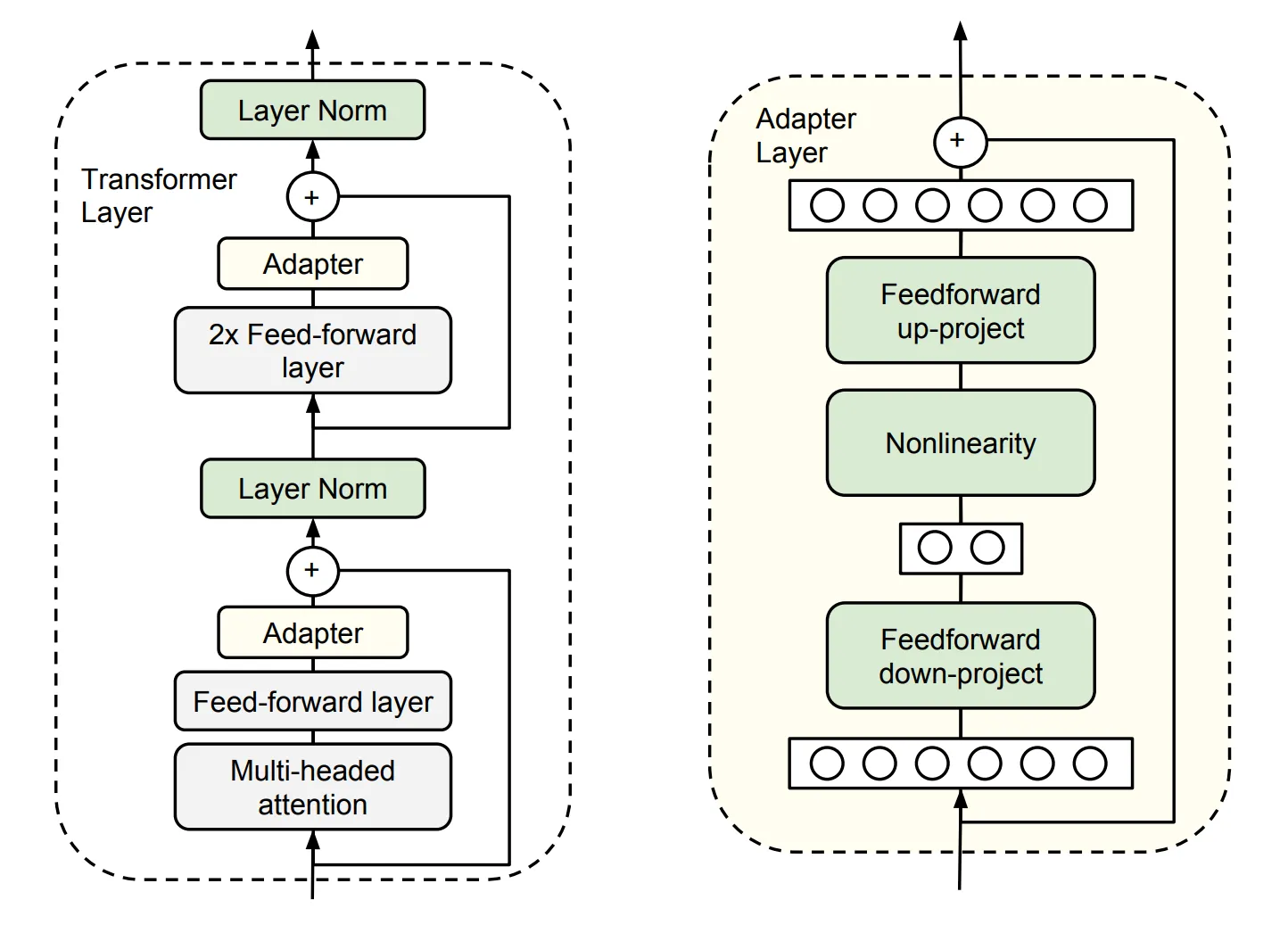
Figure 6.8 Adapt Tuning

Each Adapter module consists of two feedforward sublayers. The first feedforward sublayer takes the output of the Transformer block as input and projects the original input dimension $d$ to $m$, limiting the parameter quantity of the Adapter module by controlling $m$. Typically, $m$ is much smaller than $d$. In the output stage, the second feedforward sublayer restores the input dimension, projecting $m$ back to $d$, serving as the output of the Adapter module (as shown in the right side of the figure).

LoRA is essentially an improved version of Adapt Tuning. However, the Adapt Tuning method has a problem of increased inference latency due to the addition of extra parameters and extra computation, causing the model's calculation speed to be slower than the pre-trained model after fine-tuning.

Prefix Tuning. This method fixes the pre-trained LM and adds a trainable, task-specific prefix to the LM. This way, different tasks can save different prefixes, and the fine-tuning cost is small. Specifically, a virtual token is constructed before each input token as a prefix for the downstream task, and during fine-tuning, only the parameters of the prefix part are updated, while other parameters remain frozen.

It is also a commonly used method for light fine-tuning, known as Ptuning, which is actually an improvement of Prefix Tuning. However, Prefix Tuning also has a fixed defect: the available sequence length of the model is reduced. Due to the addition of virtual tokens, it occupies the available sequence length, so the higher the fine-tuning quality, the lower the available sequence length of the model.

6.3.2 LoRA Fine-tuning

If a large model maps data to a high-dimensional space for processing, suppose that when handling a specific small task, it is not necessary to have such a complex large model, but rather, it can be solved within a certain subspace, so there is no need to optimize all parameters. We can define that when optimizing the parameters of a certain subspace, it can reach a certain level of performance of the full parameter optimization (such as 90% accuracy), then the rank of the parameter matrix of this subspace is called the intrinsic rank of the current problem.

The pre-trained model implicitly reduces the intrinsic rank. When fine-tuning for a specific task, the weight matrix of the model actually has a lower intrinsic rank (intrinsic rank). Meanwhile, the simpler the downstream task, the lower the intrinsic rank. (Intrinsic Dimensionality Explains the Effectiveness of Language Model Fine-Tuning) Therefore, although the parameter matrix is randomly projected to a smaller subspace, it can still effectively learn, which can be understood as for a specific downstream task, these weight matrices do not require full rank. We can indirectly train some dense layers of the neural network by optimizing the rank decomposition matrix of the dense layer during adaptation, thus achieving the effect of fine-tuning by only optimizing the rank decomposition matrix of the dense layer.

For example, assuming the pre-trained parameters are $\theta^D_0$, and the intrinsic rank of the dense layer weight matrix corresponding to a specific downstream task is $\theta^d$, the fine-tuning parameters for the specific downstream task are $\theta^D$, then:

$\theta^D = \theta^D_0 + \theta^d M$

Where $M$ is the rank decomposition matrix optimized by LoRA.

Compared to other efficient fine-tuning methods, LoRA has the following advantages:

1. Small LoRA modules can be built for different downstream tasks, allowing effective switching of downstream tasks on the basis of shared pre-trained model parameters.
2. LoRA uses an adaptive optimizer (Adaptive Optimizer), which does not require computing gradients or maintaining the optimizer state of most parameters, making training more efficient and lowering hardware requirements.
3. LoRA uses a simple linear design, and during deployment, the trainable matrix is merged with the frozen weights, which does not cause inference delay.
4. LoRA is orthogonal to other methods and can be combined.

Therefore, LoRA has become the mainstream method for efficient fine-tuning of LLMs, especially in cases where resources are limited and supervised training data is limited, LoRA fine-tuning often becomes the preferred method for LLM fine-tuning.

6.3.3 Principles of LoRA Fine-tuning

(1) Low-rank Parameterized Update Matrix

LoRA assumes that there is a low intrinsic rank in the process of weight updates. For the pre-trained weight parameter matrix $W_0 \in R^{d \times k}$ (where $d$ is the output dimension of the previous layer, and $k$ is the input dimension of the next layer), it is represented by low-rank decomposition:

$$W_0 + {\Delta}W = W_0 + BA \space\space where \space B \in R^{d \times r}, A \in R^{r \times k}$$

During training, $W_0$ is frozen and not updated, while $A$ and $B$ contain trainable parameters.

Thus, the forward pass function of LoRA is:

$$h = W_0 x + \Delta W x = W_0 x + B A x$$

At the beginning of training, $A$ is initialized with random Gaussian, and $B$ is initialized with zero, and then optimized with Adam.

The training idea is shown in Figure 6.9:

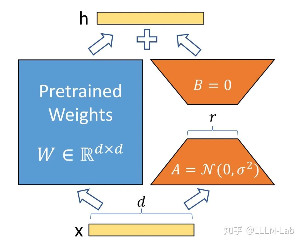
Figure 6.9 LoRA

(2) Applied to Transformer

In the Transformer architecture, LoRA technology is mainly applied to four weight matrices of the attention module: $W_q$, $W_k$, $W_v$, and $W_0$, while freezing the MLP weight matrices.

Through ablation experiments, it is found that adjusting $W_q$ and $W_v$ simultaneously produces the best results.

Under the above conditions, the number of trainable parameters is:

$\Theta = 2 \times L_{LoRA} \times d_{model} \times r$

where $L_{LoRA}$ is the number of weight matrices to which LoRA is applied, $d_{model}$ is the input and output dimension of the Transformer, and $r$ is the set LoRA rank.

Generally, $r$ is set to 4, 8, or 16.

6.3.4 Code Implementation of LoRA

Currently, the peft library is generally used to implement LoRA fine-tuning of the model. The peft library is a third-party library developed by Hugging Face, which encapsulates various efficient fine-tuning methods including LoRA, Adapt Tuning, and P-tuning, and can conveniently implement model LoRA fine-tuning.

This article briefly explains the LoRA fine-tuning code in the peft library, and analyzes the code implementation of LoRA fine-tuning.

(1) Implementation Process

The internal implementation process of LoRA fine-tuning mainly includes the following steps:

1. Determine the layers to use LoRA. The peft library currently supports three types of layers for LoRA: nn.Linear, nn.Embedding, and nn.Conv2d.

2. For each layer to be used with LoRA, replace it with a LoRA layer. What is meant by a LoRA layer is that it adds a bypass to the original result of the layer, simulating parameter updates through low-rank decomposition (i.e., matrices $A$ and $B$).

3. Freeze the original parameters and fine-tune, updating the LoRA layer parameters.

(2) Determine LoRA Layers

When performing LoRA fine-tuning, the first step is to determine the LoRA fine-tuning parameters, among which an important parameter is target_modules. target_modules is generally a list of strings, and each string is the name of a layer to be LoRA'd, for example:

target_modules = ["q_proj","v_proj"]

Here, q_proj refers to $W_q$ in the attention mechanism, and v_proj refers to $W_v$ in the attention mechanism. We can customize the layers to be LoRA'd according to the model architecture and task requirements.

When creating a LoRA model, it will obtain this parameter and find the corresponding layer in the original model. This operation is mainly implemented through regular expression matching of the layer name:

# Find the layers in the model whose names contain "q_proj", "v_proj"
target_module_found = re.fullmatch(self.peft_config.target_modules, key)
# Here, key is the component name of the model

(3) Replace LoRA Layers

For each target layer found, a new LoRA layer is created for replacement.

In terms of specific implementation, the LoRA layer is defined as a Linear class based on Lora, which inherits from both nn.Linear and LoraLayer. LoraLayer is the base class of Lora, which mainly constructs various hyperparameters of LoRA:

class LoraLayer:
    def __init__(
        self,
        r: int, # Rank of LoRA
        lora_alpha: int, # Normalization parameter
        lora_dropout: float, # Dropout ratio of LoRA layer
        merge_weights: bool, # Whether to add the LoRA matrix to the original weight matrix in evaluation mode
    ):
        self.r = r
        self.lora_alpha = lora_alpha
        # Optional dropout
        if lora_dropout > 0.0:
            self.lora_dropout = nn.Dropout(p=lora_dropout)
        else:
            self.lora_dropout = lambda x: x
        # Mark the weight as unmerged
        self.merged = False
        self.merge_weights = merge_weights
        self.disable_adapters = False

nn.Linear is the implementation of the linear layer in Pytorch. The Linear class is the specific LoRA layer, and its main implementation is as follows:

class Linear(nn.Linear, LoraLayer):
    # LoRA layer
    def __init__(
        self,
        in_features: int,
        out_features: int,
        r: int = 0,
        lora_alpha: int = 1,
        lora_dropout: float = 0.0,
        fan_in_fan_out: bool = False, 
        merge_weights: bool = True,
        **kwargs,
    ):
        # Inherit constructors of two base classes
        nn.Linear.__init__(self, in_features, out_features, **kwargs)
        LoraLayer.__init__(self, r=r, lora_alpha=lora_alpha, lora_dropout=lora_dropout, merge_weights=merge_weights)

        self.fan_in_fan_out = fan_in_fan_out
        # Actual trainable parameters
        if r > 0:
            # Parameter matrix A
            self.lora_A = nn.Linear(in_features, r, bias=False)
            # Parameter matrix B
            self.lora_B = nn.Linear(r, out_features, bias=False)
            # Normalization coefficient
            self.scaling = self.lora_alpha / self.r
            # Freeze original parameters, update only A and B
            self.weight.requires_grad = False
        # Initialize A and B
        self.reset_parameters()
        if fan_in_fan_out:
            self.weight.data = self.weight.data.T

When replacing, directly copy the weight and bias of the original layer to the new LoRA layer, and then assign the new LoRA layer to the specified device.

(4) Training

After replacing the LoRA layer, the fine-tuning training can be performed. Since the original parameters have been frozen in the LoRA layer, during training, only the parameters of A and B will be updated, thus achieving efficient fine-tuning. The overall training process is similar to the original fine-tune, and will not be detailed here. Due to the use of LoRA, the forward function will also be adjusted accordingly:

    def forward(self, x: torch.Tensor):
        if self.disable_adapters:
            if self.r > 0 and self.merged:
                self.weight.data -= (
                    transpose(self.lora_B.weight @ self.lora_A.weight, self.fan_in_fan_out) * self.scaling
                )
                self.merged = False

            return F.linear(x, transpose(self.weight, self.fan_in_fan_out), bias=self.bias)
        '''Main branch'''
        elif self.r > 0 and not self.merged:
            result = F.linear(x, transpose(self.weight, self.fan_in_fan_out), bias=self.bias)
            if self.r > 0:
                result += self.lora_B(self.lora_A(self.lora_dropout(x))) * self.scaling
            return result
        else:
            return F.linear(x, transpose(self.weight, self.fan_in_fan_out), bias=self.bias)

Due to considerations regarding parameter merging, there are several branches in the above code. Here, we only read the second branch, i.e., the elif branch. The forward calculation process based on LoRA is as described above. First, compute the product of the original parameters and the input, then add the products of A and B with the input.

6.3.5 Using peft for LoRA Fine-tuning

peft has excellent encapsulation, and supports us to conveniently and efficiently fine-tune large models. Here, we take the second section's LLM SFT as an example, and briefly introduce how to use peft to fine-tune a large model. If it is applied to RLHF, the overall idea is the same.

First, load the required libraries:

import torch.nn as nn
from transformers import AutoTokenizer, AutoModel
from peft import get_peft_model, LoraConfig, TaskType, PeftModel
from transformers import Trainer

Next, load the original model and tokenizer, which is the same as in the second section:

# Load the base model
tokenizer = AutoTokenizer.from_pretrained(MODEL_PATH, trust_remote_code=True)
model = AutoModel.from_pretrained(
    MODEL_PATH, trust_remote_code=True
)

Next, set the peft parameters:

peft_config = LoraConfig(
            task_type=TaskType.CAUSAL_LM,
            inference_mode=False,
            r=8,
            lora_alpha=32,
            lora_dropout=0.1,
        )

Note that the LoRA parameters may vary for different models. For example, for ChatGLM, it is not necessary to specify target_modeules, and peft can find them on its own; for BaiChuan, it is necessary to specify manually. task_type is the task type of the model, and large models are generally CAUSAL_LM, which is the traditional language model.

Then obtain the LoRA model:

model = get_peft_model(model, peft_config)

The underlying operation of the get_peft_model here is the specific implementation discussed above.

Finally, use the Trainer provided by Transformers for training, and the GPU memory occupied will be significantly reduced:

trainer = Trainer(
    model=model,
    args=training_args,
    train_dataset= IterableWrapper(train_dataset),
    tokenizer=tokenizer
)
trainer.train()

If it is applied to DPO or KTO, the same LoRA parameters are added and the LoRA model is obtained via get_peft_model, and no other modifications are needed. However, it should be noted that LoRA fine-tuning can significantly reduce GPU usage, and it can achieve good results in downstream task adaptation, but for tasks that require learning knowledge, LoRA, which only adjusts the low-rank matrix, is difficult to inject knowledge, and generally performs poorly, so it is not recommended to use LoRA for model pretraining or posttraining.

References

[1] Neil Houlsby, Andrei Giurgiu, Stanislaw Jastrzebski, Bruna Morrone, Quentin de Laroussilhe, Andrea Gesmundo, Mona Attariyan, and Sylvain Gelly. (2019). Parameter-Efficient Transfer Learning for NLP. arXiv preprint arXiv:1902.00751.

[2] Edward J. Hu, Yelong Shen, Phillip Wallis, Zeyuan Allen-Zhu, Yuanzhi Li, Shean Wang, Lu Wang, and Weizhu Chen. (2021). LoRA: Low-Rank Adaptation of Large Language Models. arXiv preprint arXiv:2106.09685.

[3] Armen Aghajanyan, Luke Zettlemoyer, and Sonal Gupta. (2020). Intrinsic Dimensionality Explains the Effectiveness of Language Model Fine-Tuning. arXiv preprint arXiv:2012.13255.

[4] Xiang Lisa Li and Percy Liang. (2021). Prefix-Tuning: Optimizing Continuous Prompts for Generation. arXiv preprint arXiv:2101.00190.