Transformer Architecture

2.1 Attention Mechanism

2.1.1 What is the Attention Mechanism

As NLP moved from statistical machine learning to deep learning, the method of text representation, as a core issue in NLP, gradually shifted from statistical learning to deep learning. As we introduced in Chapter 1, text representation has evolved from vector space models and language models calculated by statistical learning models, through Word2Vec's single-layer neural network, into the era of learning text representations through neural networks. However, neural networks that originated from computer vision (Computer Vision, CV) have three core architectures:

• Fully Connected Neural Network (Feedforward Neural Network, FNN), where each neuron in a layer is fully connected to every neuron in the upper and lower layers, as shown in Figure 2.1:

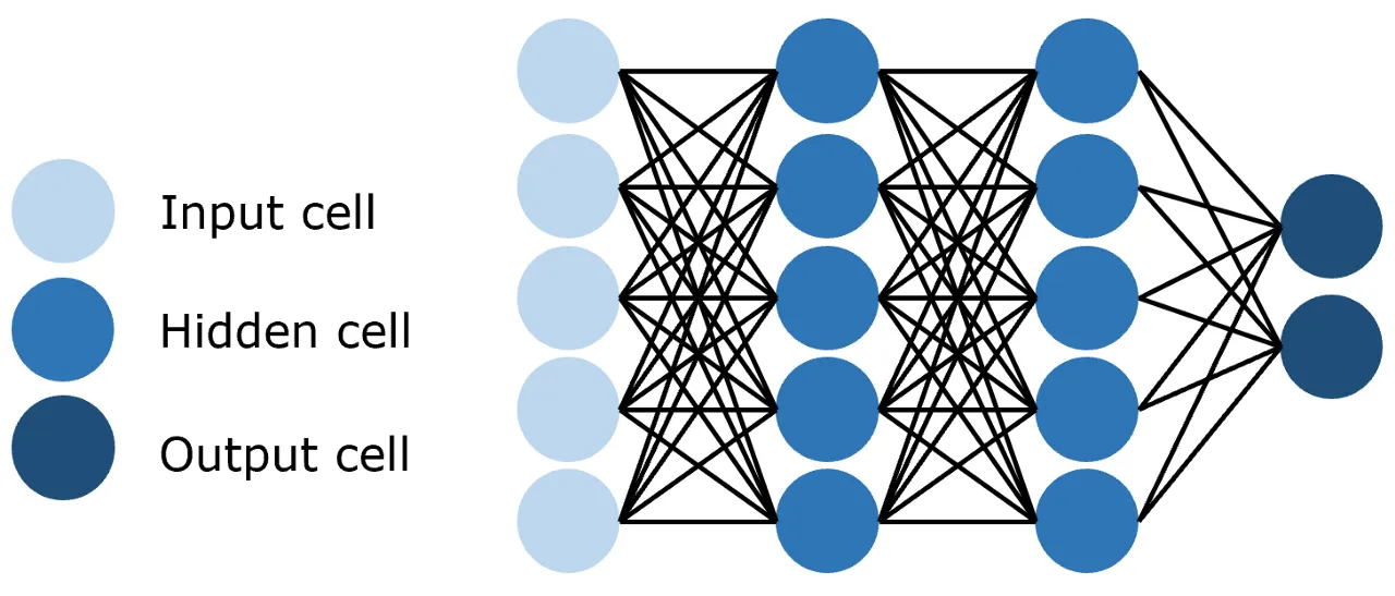
Figure 2.1 Fully Connected Neural Network

• Convolutional Neural Network (Convolutional Neural Network, CNN), which uses convolutional layers with far fewer parameters than fully connected neural networks for feature extraction and learning, as shown in Figure 2.2:

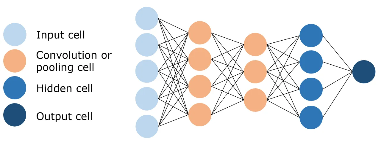
Figure 2.2 Convolutional Neural Network

• Recurrent Neural Network (Recurrent Neural Network, RNN), which can use historical information as input and contains loops and self-repetition, as shown in Figure 2.3:

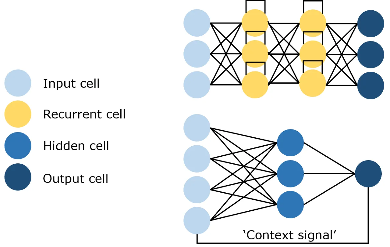
Figure 2.3 Recurrent Neural Network

Since NLP tasks often involve sequences, RNNs, which are specialized for processing sequences and time series data, often achieve optimal results in NLP tasks. In fact, before the emergence of attention mechanisms, RNNs and their derivative architecture LSTM were the undisputed kings in the field of NLP. For example, ELMo, the text representation model that pioneered the idea of pre-training, used a bidirectional LSTM as its network architecture.

However, although RNNs and LSTMs have the advantages of capturing temporal information and being suitable for sequence generation, they have two difficult-to-overcome defects:

1. The sequential calculation mode can well simulate temporal information, but limits the parallel computing capability of computers. Since sequences need to be input sequentially and calculated step by step, the parallel computing ability of the graphics processing unit (GPU) is greatly restricted, leading to high computational time costs for models based on RNNs, even though the number of parameters is not particularly large;
2. RNNs have difficulty capturing long-sequence correlations. In the RNN architecture, the farther the input is, the harder it is to capture the relationship between them. At the same time, RNNs need to read the entire sequence into memory and calculate it step by step, which also limits the length of the sequence. Although LSTM optimized this to some extent through the gate mechanism, RNNs still fall short in capturing long-distance relationships.

To address these issues, scholars such as Vaswani referred to the attention mechanism proposed in the computer vision field and frequently integrated into RNNs (note that although the attention mechanism was popularized in NLP, it was indeed first proposed in the computer vision field), and innovatively built a neural network entirely composed of attention mechanisms - Transformer, which is the ancestor and core architecture of large language models (Large Language Model, LLM), thus making attention mechanisms one of the most important architectures in deep learning.

So, what exactly is the attention mechanism?

The attention mechanism originally came from the computer vision field, and its core idea is that when we focus on an image, we do not need to see all the content clearly, but only concentrate our attention on the key parts. In natural language processing, we can also achieve more efficient and high-quality computation by focusing our attention on one or a few tokens.

The attention mechanism has three core variables: Query (query value), Key (key value), and Value (true value). We can understand the meaning of each variable through a case. For example, when we have a news report and want to find the time of the report, our Query can be a vector like "time" or "date" (for easy understanding, we use text to represent here, but in reality, it is a dense vector), and Key and Value will be the entire text. By performing operations on Query and Key, we can obtain a weight, which actually reflects the relative amount of attention that should be distributed to each token in the text from the perspective of Query. By performing operations on the weights and Value, the final result is the result of calculating the attention of the entire text from the perspective of Query.

Specifically, the characteristic of the attention mechanism is to fit the correlation between each word in the sequence by weighting the sum of the true values according to the correlation between Query and Key.

2.1.2 Understanding the Attention Mechanism Deeply

As mentioned earlier, the attention mechanism has three core variables: the query value Query, the key value Key, and the true value Value. Next, we will take a dictionary as an example to analyze how the calculation formula of the attention mechanism is derived, helping readers to deeply understand the attention mechanism. First, we have such a dictionary:

{
    "apple":10,
    "banana":5,
    "chair":2
}

At this point, the keys of the dictionary are the key values Key in the attention mechanism, and the values of the dictionary are the true values Value. The dictionary supports us to perform precise string matching. For example, if our query value Query is "apple", we can directly match it with the Key to get the corresponding Value.

However, if our Query is a concept that includes multiple Keys, for example, we want to look up "fruit", then we should match apple and banana, but not chair. Therefore, we usually choose to combine the Values corresponding to the Keys to get the final Value.

For example, when our Query is "fruit", we can assign the following weights to the three Keys:

{
    "apple":0.6,
    "banana":0.4,
    "chair":0
}

Then, the value we finally query would be:

$$value = 0.6 * 10 + 0.4 * 5 + 0 * 2 = 8$$

The different weights assigned to different Keys are called attention scores, which represent how much attention we should give to each Key in order to query the Query. However, how can we calculate the attention scores for each Query? Intuitively, we can think that the higher the relevance between the Key and the Query, the larger the attention weight it should be given. But how can we find a reasonable method to calculate the correct attention scores?

In Chapter 1, we mentioned the concept of word vectors. Through proper training, word vectors can represent semantic information, allowing semantically similar words to be closer in the vector space, and semantically distant words to be farther apart. We often use Euclidean distance to measure the similarity of word vectors, but we can also use dot product for measurement:

$$v·w = \sum_{i}v_iw_i$$

According to the definition of word vectors, the dot product of the word vectors of two semantically similar words should be greater than 0, while the dot product of the word vectors of two semantically dissimilar words should be less than 0.

Therefore, we can use the dot product to calculate the similarity between words. Assuming our Query is "fruit", corresponding to the word vector $q$; the word vectors corresponding to the Key are $k = [v_{apple} v_{banana} v_{chair}]$, then we can calculate the similarity between the Query and each key:

$$x = qK^T$$

Here, K is the matrix formed by stacking the word vectors corresponding to all Keys. According to the definition of matrix multiplication, x is the dot product of q and each k value. Now we get x, which reflects the similarity between the Query and each Key. We then convert it into weights that sum to 1 using a Softmax layer:

$$\text{softmax}(x)_i = \frac{e^{xi}}{\sum_{j}e^{x_j}}$$

This way, the resulting vector can reflect the similarity between the Query and each Key, while the sum of the weights is 1, i.e., our attention scores. Finally, we multiply the obtained attention scores with the value vectors. Based on the above process, we can obtain the basic formula for the attention mechanism calculation:

$$attention(Q,K,V) = softmax(qK^T)v$$

However, at this point, the value is still a scalar, and we only queried one Query. We can convert the value into a vector of dimension $d_v$, and query multiple Queries at the same time. Similarly, we stack the word vectors corresponding to multiple Queries into a matrix Q, and obtain the formula:

$$attention(Q,K,V) = softmax(QK^T)V$$

Currently, we are just one step away from the standard attention mechanism formula. In the previous formula, if the dimensions $d_k$ of Q and K are relatively large, the softmax scaling is very sensitive, causing significant differences between different values, thus affecting the stability of the gradient. Therefore, we need to scale the product of Q and K:

$$attention(Q,K,V) = softmax(\frac{QK^T}{\sqrt{d_k}})V$$

This is the core calculation formula of the attention mechanism.

2.1.3 Implementation of Attention Mechanism

Based on the above, we can easily implement the code for the attention mechanism using Pytorch:

'''Attention Calculation Function'''
def attention(query, key, value, dropout=None):
    '''
    args:
    query: Query Matrix
    key: Key Matrix
    value: True Value Matrix
    '''
    # Get the dimension of the key vector, which is the same as the dimension of the value vector
    d_k = query.size(-1) 
    # Calculate the inner product of Q and K and divide by the square root of dk
    # transpose —— equivalent to transposing
    scores = torch.matmul(query, key.transpose(-2, -1)) / math.sqrt(d_k)
    # Softmax
    p_attn = scores.softmax(dim=-1)
    if dropout is not None:
        p_attn = dropout(p_attn)
        # Sampling
     # Weighted sum of value based on the calculated results
    return torch.matmul(p_attn, value), p_attn

Note that in the above code, we assume that the inputs q, k, v are already converted word vector matrices, i.e., Q, K, V in the formula. We only need the above few lines of code to implement the core attention mechanism calculation.

2.1.4 Self-Attention

From the analysis above, we can see that the essence of the attention mechanism is to compute the similarity between elements of two sequences, find the correlation of each element of one sequence with each element of another sequence, and then perform weighted summation based on the correlation, i.e., allocate attention. These two sequences are the sources of Q, K, V in the calculation process.

However, in our actual application, we often only need to calculate the attention results between Query and Key, and there is rarely an additional true value Value. That is to say, we actually only need to fit two text sequences. In the classic attention mechanism, Q often comes from one sequence, and K and V come from another sequence, both calculated through parameter matrices, thereby fitting the relationship between these two sequences. For example, in the Transformer Decoder structure, Q comes from the Decoder input, and K and V come from the Encoder output, thus fitting the relationship between encoded information and historical information, facilitating the prediction of future information.

But in the Transformer Encoder structure, it uses a variant of the attention mechanism —— self-attention (self-attention). Self-attention refers to calculating the attention distribution of each element in the same sequence to other elements, that is, during the calculation process, Q, K, V are all obtained by different parameter matrices from the same input. In the Encoder, Q, K, V are respectively the products of the input with the parameter matrices $W_q、W_k、W_v$, thus fitting the relationship between each token in the input sentence and other tokens.

Through the self-attention mechanism, we can find the correlation between each token in a text and all other tokens, thus modeling the dependencies between texts. In code implementation, the self-attention mechanism is actually achieved by passing the same parameter to Q, K, V:

# attention is the attention calculation function defined above
attention(x, x, x)

2.1.5 Masked Self-Attention

Masked Self-Attention, also known as Mask Self-Attention, refers to a self-attention mechanism that uses an attention mask. The purpose of the mask is to obscure certain specific positions of the token, so that the model ignores the obscured tokens during the learning process.

The core motivation for using an attention mask is to allow the model to only use historical information for prediction without seeing future information. Transformer models that use the attention mechanism also learn through tasks similar to n-gram language models, i.e., predicting the next token based on previous tokens in a text sequence until the entire text sequence is completed.

For example, if the text sequence to be learned is 【BOS】I like you【EOS】, the model will predict and learn in the following order:

Step 1: Input 【BOS】, Output I Step 2: Input 【BOS】I, Output like Step 3: Input 【BOS】I like, Output you Step 4: Input 【BOS】I like you, Output 【EOS】

Theoretically, as long as the training corpus is sufficient, through the above process, the model can learn to model any text sequence, i.e., it can complete any text.

However, we can see that the above process is a serial process, that is, Step 1 must be completed before Step 2 can be performed, and then the entire sequence is completed step by step. We have mentioned earlier that one of the core advantages of Transformer over RNN is its ability to perform parallel calculations, which has higher computational efficiency. If for each training corpus, the model needs to perform the above process serially to complete the learning, it obviously does not achieve parallel calculation, and the computational efficiency is very low.

To address this problem, Transformer proposed the masked self-attention method. Masked self-attention generates a series of masks to obscure future information. For example, the text sequence to be learned is still 【BOS】I like you【EOS】, and the attention mask used is 【MASK】, then the model input is:

    <BOS> 【MASK】【MASK】【MASK】【MASK】
    <BOS>    I   【MASK】 【MASK】【MASK】
    <BOS>    I     like  【MASK】【MASK】
    <BOS>    I     like    you  【MASK】
    <BOS>    I     like    you   </EOS>

In each line of input, the model still only sees the previous tokens and predicts the next token. However, note that the above input is no longer a serial process, but can be input to the model in parallel. The model only needs each sample to predict the next token based on the unmasked tokens, thus achieving parallel language modeling.

Observing the above mask, we can see that it is actually an upper triangular matrix of the same length as the text sequence. We can simply create an upper triangular matrix of the same length as the input as the attention mask and then use the mask to obscure the input. That is, when the input dimension is (batch_size, seq_len, hidden_size), the mask matrix dimension is generally (1, seq_len, seq_len) (achieved through broadcasting for the same batch of different samples).

In specific implementation, we generate the mask matrix with the following code:

# Create an upper triangular matrix to obscure future information.
# First, create a 1 * seq_len * seq_len matrix using the full function
mask = torch.full((1, args.max_seq_len, args.max_seq_len), float("-inf"))
# The triu function creates an upper triangular matrix
mask = torch.triu(mask, diagonal=1)

The generated mask matrix is an upper triangular matrix, with all elements in the upper triangle set to -inf, and other positions set to 0.

During the attention calculation, we add the calculated attention scores with this mask and then perform the Softmax operation:

# Here, scores are the calculated attention scores, and mask is the mask matrix generated above
scores = scores + mask[:, :seqlen, :seqlen]
scores = F.softmax(scores.float(), dim=-1).type_as(xq)

By adding, the attention scores in the upper triangular area (i.e., the positions that should be obscured) become -inf, while the scores in the lower triangular area remain unchanged. Then, after the Softmax operation, the -inf values are set to 0, thus ignoring the attention scores calculated in the upper triangular area, thereby achieving the attention masking.

2.1.6 Multi-Head Attention

The attention mechanism can achieve parallelization and fit long-term dependencies, but a single attention calculation can only fit one type of relationship. A single attention mechanism is difficult to comprehensively fit the relationships in the sentence sequence. Therefore, Transformer uses multi-head attention mechanism (Multi-Head Attention), which performs multiple attention calculations on a corpus at the same time. Each attention calculation can fit different relationships, and the final multiple results are concatenated as the final output, thus more comprehensively and deeply fitting the language information.

In the original paper, the authors also confirmed through experiments that each different attention head can fit different information in the sentence, as shown in Figure 2.4:

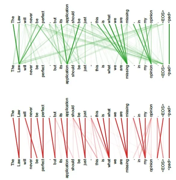
Figure 2.4 Multi-Head Attention Mechanism

The upper and lower parts are the results of self-attention calculations on the same sentence sequence by two attention heads. It can be seen that for different attention heads, different levels of related information can be fitted. By calculating simultaneously with multiple attention heads, the sentence relationships can be more comprehensively fitted.

In fact, the multi-head attention mechanism is essentially to perform multiple self-attention processes on the original input sequence; then, concatenate the self-attention results of each group, and then process them with a linear layer to obtain the final output. We can represent it with the following formula:

$$\mathrm{MultiHead}(Q, K, V) = \mathrm{Concat}(\mathrm{head_1}, ..., \mathrm{head_h})W^O \\ \text{where}~\mathrm{head_i} = \mathrm{Attention}(QW^Q_i, KW^K_i, VW^V_i)$$

Its most intuitive code implementation is not complicated, that is, n heads have n groups of three parameter matrices, each group performs the same attention calculation, but due to different parameter matrices, different attention results are achieved through backpropagation, and then the n results are concatenated and output.

However, the above implementation has high space and time complexity. We can cleverly implement parallel multi-head calculation through matrix operations. The core logic lies in using three combined matrices instead of n parameter matrix combinations. That is, matrix multiplication followed by concatenation is equivalent to concatenating matrices followed by matrix multiplication. The specific implementation can refer to the following code:

import torch.nn as nn
import torch

'''Multi-Head Self-Attention Calculation Module'''
class MultiHeadAttention(nn.Module):

    def __init__(self, args: ModelArgs, is_causal=False):
        # Constructor
        # args: configuration object
        super().__init__()
        # The hidden layer dimension must be an integer multiple of the number of heads, because we will split the input into the number of heads
        assert args.dim % args.n_heads == 0
        # The dimension of each head, equal to the model dimension divided by the total number of heads.
        self.head_dim = args.dim // args.n_heads
        self.n_heads = args.n_heads

        # Wq, Wk, Wv parameter matrices, each matrix is n_embd x dim
        # Here, we use three combined matrices to replace the combination of n parameter matrices. The logic is that matrix multiplication followed by concatenation is equivalent to concatenating matrices followed by matrix multiplication.
        # Readers who do not understand can simulate it themselves. Each linear layer is essentially the concatenation of n parameter matrices.
        self.wq = nn.Linear(args.n_embd, self.n_heads * self.head_dim, bias=False)
        self.wk = nn.Linear(args.n_embd, self.n_heads * self.head_dim, bias=False)
        self.wv = nn.Linear(args.n_embd, self.n_heads * self.head_dim, bias=False)
        # Output weight matrix, dimension is dim x dim (head_dim = dim / n_heads)
        self.wo = nn.Linear(self.n_heads * self.head_dim, args.dim, bias=False)
        # Attention dropout
        self.attn_dropout = nn.Dropout(args.dropout)
        # Residual connection dropout
        self.resid_dropout = nn.Dropout(args.dropout)
        self.is_causal = is_causal

        # Create an upper triangular matrix to obscure future information
        # Note that because it is multi-head attention, the mask matrix has one more dimension than the one we defined before
        if is_causal:
            mask = torch.full((1, 1, args.max_seq_len, args.max_seq_len), float("-inf"))
            mask = torch.triu(mask, diagonal=1)
            # Register as a buffer of the model
            self.register_buffer("mask", mask)

    def forward(self, q: torch.Tensor, k: torch.Tensor, v: torch.Tensor):

        # Get batch size and sequence length, [batch_size, seq_len, dim]
        bsz, seqlen, _ = q.shape

        # Calculate queries (Q), keys (K), and values (V), the input passes through the parameter matrix layer, dimensions are (B, T, n_embed) x (n_embed, dim) -> (B, T, dim)
        xq, xk, xv = self.wq(q), self.wk(k), self.wv(v)

        # Split Q, K, V into multiple heads, dimensions are (B, T, n_head, dim // n_head), then swap dimensions, becoming (B, n_head, T, dim // n_head)
        # Because in the attention calculation, we take the last two dimensions for calculation
        # Why first expand into B*T*n_head*C//n_head and swap the 1st and 2nd dimensions instead of directly expanding the attention input, because view expands the input directly and then constructs it according to the requirements. It can be found that only the above operation can achieve the goal of taking out the corresponding part of each head
        xq = xq.view(bsz, seqlen, self.n_heads, self.head_dim)
        xk = xk.view(bsz, seqlen, self.n_heads, self.head_dim)
        xv = xv.view(bsz, seqlen, self.n_heads, self.head_dim)
        xq = xq.transpose(1, 2)
        xk = xk.transpose(1, 2)
        xv = xv.transpose(1, 2)

        # Attention calculation
        # Calculate QK^T / sqrt(d_k), dimensions are (B, nh, T, hs) x (B, nh, hs, T) -> (B, nh, T, T)
        scores = torch.matmul(xq, xk.transpose(2, 3)) / math.sqrt(self.head_dim)
        # Masked self-attention must have an attention mask
        if self.is_causal:
            assert hasattr(self, 'mask')
            # Here, we take the sequence length, because some sequences may be shorter than max_seq_len
            scores = scores + self.mask[:, :, :seqlen, :seqlen]
        # Calculate softmax, dimensions are (B, nh, T, T)
        scores = F.softmax(scores.float(), dim=-1).type_as(xq)
        # Do Dropout
        scores = self.attn_dropout(scores)
        # V * Score, dimensions are (B, nh, T, T) x (B, nh, T, hs) -> (B, nh, T, hs)
        output = torch.matmul(scores, xv)

        # Restore the time dimension and concatenate the heads.
        # Concatenate the results of multiple heads, first swap the dimensions to (B, T, n_head, dim // n_head), then concatenate to (B, T, n_head * dim // n_head)
        # contiguous function is used to re-allocate a new memory storage, because Pytorch sets that after transpose and view, an error occurs,
        # because view is based on the underlying storage, and transpose does not change the underlying storage, so an extra storage is needed
        output = output.transpose(1, 2).contiguous().view(bsz, seqlen, -1)

        # Finally project back to residual stream.
        output = self.wo(output)
        output = self.resid_dropout(output)
        return output

2.2 Encoder-Decoder

In the previous section, we detailed the core of Transformer —— the attention mechanism. In the paper "Attention is All You Need," the authors built the Transformer model by using only the attention mechanism and discarding traditional RNN and CNN architectures, thus bringing a revolution to the field of NLP. In Transformer, the two core components are the Encoder (encoder) and Decoder (decoder), which use the attention mechanism. In fact, subsequent pre-trained language models based on the Transformer architecture are mostly improved by modifying the Encoder-Decoder part to build new model architectures, such as BERT which uses only the Encoder and GPT which uses only the Decoder.

In this section, we will start from the Seq2Seq task that Transformer is aimed at, and analyze the Encoder-Decoder structure of Transformer based on the attention mechanism introduced in the previous section.

2.2.1 Seq2Seq Model

Seq2Seq, short for Sequence to Sequence, is a classic NLP task. Specifically, it refers to a model where the input is a natural language sequence $input = (x_1, x_2, x_3...x_n)$, and the output is a possibly unequal-length natural language sequence $output = (y_1, y_2, y_3...y_m)$. In fact, Seq2Seq is the most classic task in NLP, and almost all NLP tasks can be considered as Seq2Seq tasks. For example, text classification tasks can be considered as target sequences with a length of 1 (such as in the above equation, $m$ = 1); part-of-speech tagging tasks can be considered as target sequences with the same length as the input sequence (such as in the above equation, $m$ = $n$).

Machine translation is a classic Seq2Seq task, for example, the input might be "Today's weather is nice," and the output is "Today is a good day." Transformer is a classic Seq2Seq model, meaning that the input of the model is a text sequence, and the output is another text sequence. In fact, Transformer was initially applied to the task of machine translation.

For Seq2Seq tasks, the general approach is to encode the natural language sequence and then decode it. Encoding refers to encoding the input natural language sequence into a vector (or matrix) that represents semantics, which can be simply understood as a more complex word vector representation. Decoding refers to outputting the vector or matrix encoded from the input natural language sequence through the hidden layer, and then decoding it into the corresponding natural language target sequence. Through encoding and decoding, the Seq2Seq task can be achieved.

The Encoder in Transformer is used for the above encoding process; the Decoder is used for the above decoding process. The Transformer structure, as shown in Figure 2.5:

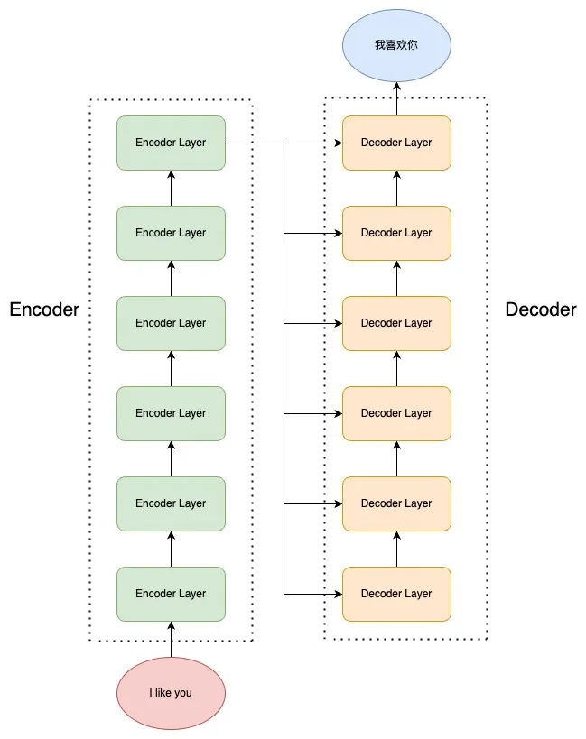
Figure 2.5 Encoder-Decoder Structure

Transformer consists of an Encoder and a Decoder, and each Encoder (Decoder) is composed of 6 Encoder (Decoder) Layers. The source sequence enters the Encoder for encoding, and the encoded result is output to each layer of the Decoder Layer at the top of the Encoder Layer, and after decoding by the Decoder, the output target sequence can be obtained.

Next, we will first introduce the classical neural network structures within the Encoder and Decoder —— the feed-forward neural network (FNN), layer normalization (Layer Norm), and residual connection (Residual Connection), and then further analyze the internal structure of the Encoder and Decoder.

2.2.2 Feed-Forward Neural Network

The feed-forward neural network (Feed Forward Neural Network, abbreviated as FNN), which we mentioned in the previous section, is a network structure where each neuron in a layer is fully connected to every neuron in the upper and lower layers. Each Encoder Layer contains the attention mechanism mentioned above and a feed-forward neural network. The implementation of the feed-forward neural network is relatively simple:

class MLP(nn.Module):
    '''Feed Forward Neural Network'''
    def __init__(self, dim: int, hidden_dim: int, dropout: float):
        super().__init__()
        # Define the first linear transformation from input dimension to hidden dimension
        self.w1 = nn.Linear(dim, hidden_dim, bias=False)
        # Define the second linear transformation from hidden dimension to input dimension
        self.w2 = nn.Linear(hidden_dim, dim, bias=False)
        # Define a dropout layer to prevent overfitting
        self.dropout = nn.Dropout(dropout)

    def forward(self, x):
        # Forward propagation function
        # First, the input x passes through the first linear transformation and the RELU activation function
        # Finally, it passes through the second linear transformation and the dropout layer
        return self.dropout(self.w2(F.relu(self.w1(x))))
    

Note that the feed-forward neural network in Transformer consists of two linear layers with a RELU activation function in between, and also includes a Dropout layer to prevent overfitting.

2.2.3 Layer Normalization

Layer Normalization, also known as Layer Norm, is a classic normalization operation in deep learning. The mainstream normalization in neural networks generally has two types: Batch Normalization (Batch Norm) and Layer Normalization (Layer Norm).

Normalization is essentially to make the input values or distributions of different layers more consistent. Since the input of each layer in a deep neural network is the output of the previous layer, with multiple layers, the distribution of the inputs of higher layers changes significantly due to the parameter changes of all previous neural layers. That is to say, as the parameters of the neural network update, the output distributions of each layer are different, and the difference increases with the depth of the network. However, the conditional distribution to be predicted remains the same, thus causing prediction errors.

Therefore, in deep neural networks, normalization operations are often needed to normalize the inputs of each layer into a standard normal distribution. Batch Normalization refers to normalization on a mini-batch, which is equivalent to splitting out a portion of the samples in a batch, first calculating the mean of the samples:

$$\mu_j = \frac{1}{m}\sum^{m}_{i=1}Z_j^{i}$$

where $Z_j^{i}$ is the value of sample i on the j-th dimension, and m is the size of the mini-batch.

Then calculate the variance of the samples:

$$\sigma^2 = \frac{1}{m}\sum^{m}_{i=1}(Z_j^i - \mu_j)^2$$

Finally, subtract the mean and divide by the standard deviation to convert the distribution of the samples in the mini-batch into a standard normal distribution:

$$\widetilde{Z_j} = \frac{Z_j - \mu_j}{\sqrt{\sigma^2 + \epsilon}}$$

Here, adding $\epsilon$ is to avoid division by zero.

However, Batch Normalization has some defects, such as:

• When the GPU memory is limited and the mini-batch is small, the mean and variance taken by Batch Norm cannot reflect the global statistical distribution information, thus leading to poor performance;
• For RNNs expanded in the time dimension, the same distribution of different sentences is probably different, so Batch Norm normalization loses meaning;
• During training, Batch Norm needs to save the statistical information (mean and variance) for each step. During testing, due to the characteristics of variable-length sentences, the test set may have longer sentences than the training set, so for later steps, there is no statistical information available for training;
• Applying Batch Norm requires saving and calculating batch statistics for each step, which is time-consuming and resource-intensive

Therefore, Layer Normalization, which is more commonly used and more effective in deep neural networks, was introduced. Compared to Batch Norm, which calculates the mean and variance of all samples in each layer, Layer Norm calculates the mean and variance of all layers for each sample, thus stabilizing the distribution of each sample. The normalization method of Layer Norm is completely the same as that of Batch Norm, except for the different dimensions of statistical quantities.

Based on the above normalization formula, we can simply implement a Layer Norm layer:

class LayerNorm(nn.Module):
    ''' Layer Norm Layer'''
    def __init__(self, features, eps=1e-6):
	super().__init__()
    # Linear matrix for mapping
	self.a_2 = nn.Parameter(torch.ones(features))
	self.b_2 = nn.Parameter(torch.zeros(features))
	self.eps = eps
	
    def forward(self, x):
	# Calculate the mean and variance of all dimensions of each sample
	mean = x.mean(-1, keepdim=True) # mean: [bsz, max_len, 1]
	std = x.std(-1, keepdim=True) # std: [bsz, max_len, 1]
    # Note that here the broadcast occurs on the last dimension
	return self.a_2 * (x - mean) / (std + self.eps) + self.b_2

Note that in the Layer Norm layer we implemented above, there are two linear matrices for mapping.

2.2.4 Residual Connection

Due to the complex structure and deep layers of the Transformer model, to avoid model degradation, the Transformer adopted the idea of residual connections to connect each sub-layer. A residual connection means that the input of the next layer is not only the output of the previous layer, but also includes the input of the previous layer. The residual connection allows the information from the bottom layer to be directly passed to the top layer, letting the upper layer focus on learning the residual.

For example, in the Encoder, in the first sub-layer, the input enters the multi-head self-attention layer while directly passing to the output of that layer, and then the output of that layer is added to the original input, and then normalized. In the second sub-layer, it is the same. That is:

$$x = x + MultiHeadSelfAttention(LayerNorm(x))$$ $$output = x + FNN(LayerNorm(x))$$

In our code implementation, we achieve the residual connection by adding the original value in the forward calculation of the layer:

# Attention calculation
h = x + self.attention.forward(self.attention_norm(x))
# After the feed-forward neural network
out = h + self.feed_forward.forward(self.fnn_norm(h))

In the above code, self.attention_norm and self.fnn_norm are both LayerNorm layers, self.attn is the attention layer, and self.feed_forward is the feed-forward neural network.

2.2.5 Encoder

After implementing the above components, we can build the Transformer Encoder. The Encoder is composed of N Encoder Layers, each Encoder Layer includes an attention layer and a feed-forward neural network. Therefore, we can first implement an Encoder Layer:

class EncoderLayer(nn.Module):
  '''Encoder Layer'''
    def __init__(self, args):
        super().__init__()
        # There are two LayerNorms in a Layer, one before the Attention and one before the MLP
        self.attention_norm = LayerNorm(args.n_embd)
        # Encoder does not need a mask, pass is_causal=False
        self.attention = MultiHeadAttention(args, is_causal=False)
        self.fnn_norm = LayerNorm(args.n_embd)
        self.feed_forward = MLP(args.dim, args.dim, args.dropout)

    def forward(self, x):
        # Layer Norm
        norm_x = self.attention_norm(x)
        # Self-attention
        h = x + self.attention.forward(norm_x, norm_x, norm_x)
        # Feed-forward neural network
        out = h + self.feed_forward.forward(self.fnn_norm(h))
        return out

Then we build an Encoder composed of N Encoder Layers, and finally add a Layer Norm to achieve normalization:

class Encoder(nn.Module):
    '''Encoder Block'''
    def __init__(self, args):
        super(Encoder, self).__init__() 
        # An Encoder is composed of N Encoder Layers
        self.layers = nn.ModuleList([EncoderLayer(args) for _ in range(args.n_layer)])
        self.norm = LayerNorm(args.n_embd)

    def forward(self, x):
        "Pass through N Encoder Layers"
        for layer in self.layers:
            x = layer(x)
        return self.norm(x)

The output of the Encoder is the result of encoding the input.

2.2.6 Decoder

Similarly, we can first build a Decoder Layer, and then assemble N Decoder Layers into a Decoder. However, unlike the Encoder, the Decoder consists of two attention layers and a feed-forward neural network. The first attention layer is a masked self-attention layer, i.e., using masked attention calculation to ensure that each token can only use the attention scores before that token; the second attention layer is a multi-head attention layer, which uses the output of the first attention layer as the query, and the output of the Encoder as the key and value, to calculate the attention scores. Finally, it goes through the feed-forward neural network:

class DecoderLayer(nn.Module):
  '''Decoder Layer'''
    def __init__(self, args):
        super().__init__()
        # There are three LayerNorms in a Layer, one before the Mask Attention, one before the Self Attention, and one before the MLP
        self.attention_norm_1 = LayerNorm(args.n_embd)
        # The first part of the Decoder is Mask Attention, pass is_causal=True
        self.mask_attention = MultiHeadAttention(args, is_causal=True)
        self.attention_norm_2 = LayerNorm(args.n_embd)
        # The second part of the Decoder is similar to the Encoder's Attention, pass is_causal=False
        self.attention = MultiHeadAttention(args, is_causal=False)
        self.ffn_norm = LayerNorm(args.n_embd)
        # The third part is MLP
        self.feed_forward = MLP(args.dim, args.dim, args.dropout)

    def forward(self, x, enc_out):
        # Layer Norm
        norm_x = self.attention_norm_1(x)
        # Masked self-attention
        x = x + self.mask_attention.forward(norm_x, norm_x, norm_x)
        # Multi-head attention
        norm_x = self.attention_norm_2(x)
        h = x + self.attention.forward(norm_x, enc_out, enc_out)
        # Feed-forward neural network
        out = h + self.feed_forward.forward(self.ffn_norm(h))
        return out

Then, similarly, we build a Decoder block:

class Decoder(nn.Module):
    '''Decoder'''
    def __init__(self, args):
        super(Decoder, self).__init__() 
        # A Decoder is composed of N Decoder Layers
        self.layers = nn.ModuleList([DecoderLayer(args) for _ in range(args.n_layer)])
        self.norm = LayerNorm(args.n_embd)

    def forward(self, x, enc_out):
        "Pass the input (and mask) through each layer in turn."
        for layer in self.layers:
            x = layer(x, enc_out)
        return self.norm(x)

After completing the construction of the Encoder and Decoder, we have completed the core part of the Transformer. Next, we can assemble the Encoder and Decoder and add the Embedding layer to build the complete Transformer model.

2.3 Building a Transformer

In the previous two chapters, we analyzed in detail the attention mechanism and the core of Transformer —— the Encoder and Decoder structures. Next, we can build a complete Transformer model based on the components implemented in the previous chapter.

2.3.1 Embedding Layer

As we mentioned in Chapter 1, in NLP tasks, we often need to convert natural language input into vectors that machines can process. The component responsible for this task in deep learning is the Embedding layer.

The Embedding layer is essentially an embedding lookup table that stores fixed-size dictionaries of vectors. That is, before feeding the input into the neural network, we usually let the natural language input go through a tokenizer, whose role is to split the natural language input into tokens and convert them into fixed indexes. For example, if we set the vocabulary size to 4, and the input is "I like you," the tokenizer can convert the input into:

input: I
output: 0

input: like
output: 1

input: you
output: 2

Of course, in practice, the work of the tokenizer is more complex. For example, tokenization can be done in various ways, such as splitting into words, subwords, or characters, and the vocabulary size is often as high as tens of thousands. Here we do not elaborate on the details of the tokenizer, and will introduce how the tokenizer of large models works and is trained in the following sections.

Therefore, the input of the Embedding layer is usually a matrix with shape (batch_size, seq_len, 1), where the first dimension is the number of batches, the second dimension is the length of the natural language sequence, and the third dimension is the index value of the token after being converted by the tokenizer. For example, for the above input, the input of the Embedding layer would be:

[[[0],[1],[2]]]

with a batch_size of 1 and a seq_len of 3, and the converted indexes as above.

The Embedding layer itself is actually a trainable (Vocab_size, embedding_dim) weight matrix, where each value in the vocabulary corresponds to a row of a vector with dimension embedding_dim. For the input values, they correspond to these word vectors, and are concatenated into a matrix of (batch_size, seq_len, embedding_dim) as output.

This implementation is not complicated, and we can directly use the Embedding layer in torch:

self.tok_embeddings = nn.Embedding(args.vocab_size, args.dim)

2.3.2 Positional Encoding

The attention mechanism enables good parallel computing, but it also leads to the loss of relative positions in the sequence. In RNNs and LSTMs, the input sequence is processed recursively in the order of the sentence, so the order of the input sequence provides extremely important information, which is also very consistent with the characteristics of natural language.

However, from the analysis of the attention mechanism in the previous section, we can see that in the calculation process of the attention mechanism, each token in the sequence is treated equally, i.e., "I like you" and "you like me" are considered the same in the attention mechanism, but this is a major problem with the attention mechanism. Therefore, to use the sequence order information and retain the relative position information in the sequence, Transformer adopts a positional encoding mechanism, which has been used by many models afterward.

Positional encoding refers to encoding the relative position of tokens in the sequence and then adding the positional encoding to the word vector encoding. There are many ways to perform positional encoding, and Transformer uses sinusoidal functions for positional encoding (absolute positional encoding), with the encoding method as follows:

$$PE(pos, 2i) = sin(pos/10000^{2i/d_{model}})\\ PE(pos, 2i+1) = cos(pos/10000^{2i/d_{model}})$$

In the above formula, pos is the position of the token in the sentence, and 2i and 2i+1 indicate whether the token is in an odd or even position. From the formula, we can see that for odd-positioned tokens and even-positioned tokens, Transformer uses different functions for encoding.

We will illustrate the calculation process of positional encoding with a simple example. Suppose we input a sentence of length 4 "I like to code," we can get the following word vector matrix $\rm x$, where each row represents a word vector, $\rm x_0=[0.1,0.2,0.3,0.4]$ corresponds to the word "I," and its pos is 0, and so on, the second row represents the word vector of "like," and its pos is 1:

$$\rm x = \begin{bmatrix} 0.1 & 0.2 & 0.3 & 0.4 \\ 0.2 & 0.3 & 0.4 & 0.5 \\ 0.3 & 0.4 & 0.5 & 0.6 \\ 0.4 & 0.5 & 0.6 & 0.7 \end{bmatrix}$$

Then, the word vectors after positional encoding are:

$$\rm x_{PE} = \begin{bmatrix} 0.1 & 0.2 & 0.3 & 0.4 \\ 0.2 & 0.3 & 0.4 & 0.5 \\ 0.3 & 0.4 & 0.5 & 0.6 \\ 0.4 & 0.5 & 0.6 & 0.7 \end{bmatrix} + \begin{bmatrix} \sin(\frac{0}{10000^0}) & \cos(\frac{0}{10000^0}) & \sin(\frac{0}{10000^{2/4}}) & \cos(\frac{0}{10000^{2/4}}) \\ \sin(\frac{1}{10000^0}) & \cos(\frac{1}{10000^0}) & \sin(\frac{1}{10000^{2/4}}) & \cos(\frac{1}{10000^{2/4}}) \\ \sin(\frac{2}{10000^0}) & \cos(\frac{2}{10000^0}) & \sin(\frac{2}{10000^{2/4}}) & \cos(\frac{2}{10000^{2/4}}) \\ \sin(\frac{3}{10000^0}) & \cos(\frac{3}{10000^0}) & \sin(\frac{3}{10000^{2/4}}) & \cos(\frac{3}{10000^{2/4}}) \end{bmatrix} = \begin{bmatrix} 0.1 & 1.2 & 0.3 & 1.4 \\ 1.041 & 0.84 & 0.41 & 1.49 \\ 1.209 & -0.016 & 0.52 & 1.59 \\ 0.541 & -0.489 & 0.895 & 1.655 \end{bmatrix}$$

We can use the following code to obtain the positional encoding in the above example:

import numpy as np
import matplotlib.pyplot as plt
def PositionEncoding(seq_len, d_model, n=10000):
    P = np.zeros((seq_len, d_model))
    for k in range(seq_len):
        for i in np.arange(int(d_model/2)):
            denominator = np.power(n, 2*i/d_model)
            P[k, 2*i] = np.sin(k/denominator)
            P[k, 2*i+1] = np.cos(k/denominator)
    return P

P = PositionEncoding(seq_len=4, d_model=4, n=100)
print(P)

[[ 0.          1.          0.          1.        ]
 [ 0.84147098  0.54030231  0.09983342  0.99500417]
 [ 0.90929743 -0.41614684  0.19866933  0.98006658]
 [ 0.14112001 -0.9899925   0.29552021  0.95533649]]

This kind of positional encoding has two main benefits:

1. It allows PE to adapt to sentences longer than those in the training set. Suppose the longest sentence in the training set has 20 words, and suddenly a sentence of 21 words appears, then the method of calculating using the formula can calculate the embedding for the 21st position.
2. It allows the model to easily calculate the relative position. For a fixed distance k, PE(pos+k) can be calculated from PE(pos). Because Sin(A+B) = Sin(A)Cos(B) + Cos(A)Sin(B), Cos(A+B) = Cos(A)Cos(B) - Sin(A)Sin(B).

We can also rigorously prove the superiority of this encoding method through mathematical derivation. The original Transformer Embedding can be represented as:

$$\begin{equation}f(\cdots,\boldsymbol{x}_m,\cdots,\boldsymbol{x}_n,\cdots)=f(\cdots,\boldsymbol{x}_n,\cdots,\boldsymbol{x}_m,\cdots)\end{equation}$$

It is obvious that this function is not asymmetric, i.e., it cannot represent relative position information. We want to get such an encoding method:

$$\begin{equation}\tilde{f}(\cdots,\boldsymbol{x}_m,\cdots,\boldsymbol{x}_n,\cdots)=f(\cdots,\boldsymbol{x}_m + \boldsymbol{p}_m,\cdots,\boldsymbol{x}_n + \boldsymbol{p}_n,\cdots)\end{equation}$$

Here, the added $p_m$, $p_n$ are the position encodings. Next, we will perform a Taylor expansion of $f(...,x_m+p_m,...,x_n+p_n)$ at positions m and n:

$$\begin{equation}\tilde{f}\approx f + \boldsymbol{p}_m^{\top} \frac{\partial f}{\partial \boldsymbol{x}_m} + \boldsymbol{p}_n^{\top} \frac{\partial f}{\partial \boldsymbol{x}_n} + \frac{1}{2}\boldsymbol{p}_m^{\top} \frac{\partial^2 f}{\partial \boldsymbol{x}_m^2}\boldsymbol{p}_m + \frac{1}{2}\boldsymbol{p}_n^{\top} \frac{\partial^2 f}{\partial \boldsymbol{x}_n^2}\boldsymbol{p}_n + \underbrace{\boldsymbol{p}_m^{\top} \frac{\partial^2 f}{\partial \boldsymbol{x}_m \partial \boldsymbol{x}_n}\boldsymbol{p}_n}_{\boldsymbol{p}_m^{\top} \boldsymbol{\mathcal{H}} \boldsymbol{p}_n}\end{equation}$$

It can be seen that the first term is unrelated to the position, the second to fifth terms depend only on a single position, and the sixth term (f is partially differentiated with respect to m and n) is related to two positions, so we hope the sixth term ($p_m^THp_n$) expresses the relative position information, i.e., find a function g such that:

$$p_m^THp_n = g(m-n)$$

We assume that $H$ is an identity matrix, then:

$$p_m^THp_n = p_m^Tp_n = \langle\boldsymbol{p}_m, \boldsymbol{p}_n\rangle = g(m-n)$$

By treating the vector [x,y] as a complex number x+yi, and building equations based on the rules of complex numbers:

$$\begin{equation}\langle\boldsymbol{p}_m, \boldsymbol{p}_n\rangle = \text{Re}[\boldsymbol{p}_m \boldsymbol{p}_n^*]\end{equation}$$

Then assuming there exists a complex number $q_{m-n}$ such that:

$$\begin{equation}\boldsymbol{p}_m \boldsymbol{p}_n^* = \boldsymbol{q}_{m-n}\end{equation}$$

Solving this equation using the exponential form of complex numbers, we get the solution for the two-dimensional position encoding:

$$\begin{equation}\boldsymbol{p}_m = e^{\text{i}m\theta}\quad\Leftrightarrow\quad \boldsymbol{p}_m=\begin{pmatrix}\cos m\theta \\ \sin m\theta\end{pmatrix}\end{equation}$$

Since the inner product satisfies linear superposition, the higher-dimensional even-dimensional position encoding can be represented as a combination of multiple two-dimensional position encodings:

$$\begin{equation}\boldsymbol{p}_m = \begin{pmatrix}e^{\text{i}m\theta_0} \\ e^{\text{i}m\theta_1} \\ \vdots \\ e^{\text{i}m\theta_{d/2-1}}\end{pmatrix}\quad\Leftrightarrow\quad \boldsymbol{p}_m=\begin{pmatrix}\cos m\theta_0 \\ \sin m\theta_0 \\ \cos m\theta_1 \\ \sin m\theta_1 \\ \vdots \\ \cos m\theta_{d/2-1} \\ \sin m\theta_{d/2-1} \end{pmatrix}\end{equation}$$

Then take $\theta_i = 10000^{-2i/d}$ (this form makes the ⟨pm,pn⟩ tend to zero as |m−n| increases, which can be proven by integrating the position encoding, and the base is 10000 as an experimental result), we get the above encoding method.

When $H$ is not an identity matrix, since the correlation between any two dimensions of the d-dimensional vectors formed by the model's Embedding layer is small and has a certain decoupling property, we can consider it as a diagonal matrix. Then using the above encoding:

$$\begin{equation}\boldsymbol{p}_m^{\top} \boldsymbol{\mathcal{H}} \boldsymbol{p}_n=\sum_{i=1}^{d/2} \boldsymbol{\mathcal{H}}_{2i,2i} \cos m\theta_i \cos n\theta_i + \boldsymbol{\mathcal{H}}_{2i+1,2i+1} \sin m\theta_i \sin n\theta_i\end{equation}$$

Using the product-to-sum formula:

$$\begin{equation}\sum_{i=1}^{d/2} \frac{1}{2}\left(\boldsymbol{\mathcal{H}}_{2i,2i} + \boldsymbol{\mathcal{H}}_{2i+1,2i+1}\right) \cos (m-n)\theta_i + \frac{1}{2}\left(\boldsymbol{\mathcal{H}}_{2i,2i} - \boldsymbol{\mathcal{H}}_{2i+1,2i+1}\right) \cos (m+n)\theta_i \end{equation}$$

This shows that the encoding can still represent the relative position.

The above encoding results, as shown in Figure 2.6:

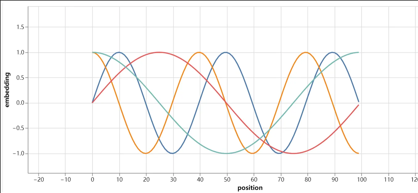
Figure 2.6 Encoding Results

Based on the above principles, we implement a positional encoding layer:

class PositionalEncoding(nn.Module):
    '''Positional Encoding Module'''

    def __init__(self, args):
        super(PositionalEncoding, self).__init__()
        # Dropout layer
        # self.dropout = nn.Dropout(p=args.dropout)

        # block size is the maximum length of the sequence
        pe = torch.zeros(args.block_size, args.n_embd)
        position = torch.arange(0, args.block_size).unsqueeze(1)
        # Calculate theta
        div_term = torch.exp(
            torch.arange(0, args.n_embd, 2) * -(math.log(10000.0) / args.n_embd)
        )
        # Calculate sin and cos results separately
        pe[:, 0::2] = torch.sin(position * div_term)
        pe[:, 1::2] = torch.cos(position * div_term)
        pe = pe.unsqueeze(0)
        self.register_buffer("pe", pe)

    def forward(self, x):
        # Add positional encoding to the Embedding result
        x = x + self.pe[:, : x.size(1)].requires_grad_(False)
        return x

2.3.3 A Complete Transformer

All the above components, when assembled according to the Transformer structure shown in the following figure, form a complete Transformer model, as shown in Figure 2.7:

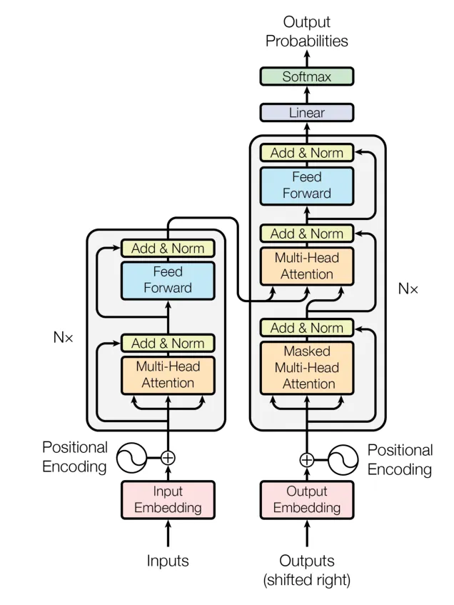
Figure 2.7 Transformer Model Structure

However, it should be noted that the above figure is the diagram from the original paper "Attention is all you need," where the LayerNorm layer is placed after the Attention layer, i.e., the "Post-Norm" structure. However, in the source code released by the paper, the LayerNorm layer is placed before the Attention layer, i.e., the "Pre-Norm" structure. Considering that current LLMs generally adopt the "Pre-Norm" structure (which can make the loss more stable), the implementation in this article adopts the "Pre-Norm" structure.

As shown in the figure, after the tokenizer mapping, the output first goes through the Embedding layer and the Positional Embedding layer, then enters the N Encoder and N Decoder (in the original Transformer model, N is set to 6), and finally, after a linear layer and a Softmax layer, the final output is obtained.

Based on the components we have implemented, we implement the complete Transformer model:

class Transformer(nn.Module):
   '''Whole Model'''
    def __init__(self, args):
        super().__init__()
        # Must input vocabulary size and block size
        assert args.vocab_size is not None
        assert args.block_size is not None
        self.args = args
        self.transformer = nn.ModuleDict(dict(
            wte = nn.Embedding(args.vocab_size, args.n_embd),
            wpe = PositionalEncoding(args),
            drop = nn.Dropout(args.dropout),
            encoder = Encoder(args),
            decoder = Decoder(args),
        ))
        # Final linear layer, input is n_embd, output is vocabulary size
        self.lm_head = nn.Linear(args.n_embd, args.vocab_size, bias=False)

        # Initialize all weights
        self.apply(self._init_weights)

        # Count the number of parameters
        print("number of parameters: %.2fM" % (self.get_num_params()/1e6,))

    '''Count the number of parameters'''
    def get_num_params(self, non_embedding=False):
        # non_embedding: whether to count the embedding parameters
        n_params = sum(p.numel() for p in self.parameters())
        # If not counting the embedding parameters, subtract
        if non_embedding:
            n_params -= self.transformer.wte.weight.numel()
        return n_params

    '''Initialize weights'''
    def _init_weights(self, module):
        # Initialize linear layers and Embedding layers with normal distribution
        if isinstance(module, nn.Linear):
            torch.nn.init.normal_(module.weight, mean=0.0, std=0.02)
            if module.bias is not None:
                torch.nn.init.zeros_(module.bias)
        elif isinstance(module, nn.Embedding):
            torch.nn.init.normal_(module.weight, mean=0.0, std=0.02)
    
    '''Forward calculation function'''
    def forward(self, idx, targets=None):
        # Input is idx, with dimension (batch size, sequence length, 1); targets are the target sequence, used to calculate loss
        device = idx.device
        b, t = idx.size()
        assert t <= self.args.block_size, f"Cannot calculate this sequence, the sequence length is {t}, the maximum sequence length is only {self.args.block_size}"

        # Through self.transformer
        # First, pass the input idx through the Embedding layer, getting a dimension of (batch size, sequence length, n_embd)
        print("idx",idx.size())
        # Through the Embedding layer
        tok_emb = self.transformer.wte(idx)
        print("tok_emb",tok_emb.size())
        # Then through positional encoding
        pos_emb = self.transformer.wpe(tok_emb) 
        # Then apply Dropout
        x = self.transformer.drop(pos_emb)
        # Then through Encoder
        print("x after wpe:",x.size())
        enc_out = self.transformer.encoder(x)
        print("enc_out:",enc_out.size())
        # Then through Decoder
        x = self.transformer.decoder(x, enc_out)
        print("x after decoder:",x.size())

        if targets is not None:
            # Training phase, if we provide targets, calculate loss
            # First, pass through the final linear layer, getting a dimension of (batch size, sequence length, vocab size)
            logits = self.lm_head(x)
            # Then calculate cross-entropy with targets
            loss = F.cross_entropy(logits.view(-1, logits.size(-1)), targets.view(-1), ignore_index=-1)
        else:
            # Inference phase, we only need logits, loss is None
            # Take -1 to preserve the time dimension
            logits = self.lm_head(x[:, [-1], :]) # note: using list [-1] to preserve the time dim
            loss = None

        return logits, loss

Note that in addition to building the entire Transformer structure, the above code also implements three functions:

• get_num_params: used to count the number of model parameters
• _init_weights: used to randomly initialize all model parameters
• forward: the forward calculation function

In addition, in the forward calculation function, we use Pytorch's cross-entropy function to calculate the loss. For different loss functions, readers can refer to the Pytorch official documentation, and we will not elaborate further here.

After the above steps, we can build a complete, computable Transformer model from scratch. Due to the focus of this book on LLM, we will not elaborate on how to train the Transformer model in this chapter; in the following sections, we will similarly build a LLaMA model from scratch and guide you to train your own Tiny LLaMA.

References

[1] Ashish Vaswani, Noam Shazeer, Niki Parmar, Jakob Uszkoreit, Llion Jones, Aidan N. Gomez, Lukasz Kaiser, Illia Polosukhin. (2023). Attention Is All You Need. arXiv preprint arXiv:1706.03762.

[2] Jay Mody's article "An Intuition for Attention". Source: https://jaykmody.com/blog/attention-intuition/